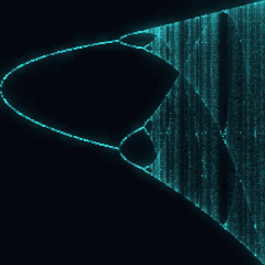
Logistic Bifurcation Diagram

DEFINITION

xₙ₊₁ = r·xₙ(1 − xₙ)
plotted against r, transient discarded
Feigenbaum δ = 4.6692016091… (ratio of successive doubling intervals)

NOTES

Verhulst wrote this in 1838 to correct Malthus — unbounded growth cannot be right, so he multiplied it by a term that falls to zero as the population fills its room. For a century and a half it was read as a population model and nothing else. What it does past r ≈ 3 sat unremarked: turn the growth rate up and the settled population stops being one value and splits into a two-cycle, then four, then eight, each split arriving sooner than the last, until past r ≈ 3.56995 it never settles at all. The May 1976 Nature paper made that cascade famous, as a warning against assuming a simple equation must behave simply. Feigenbaum found the actual content in it two years later: the ratio by which each doubling interval shrinks relative to the one before it converges to δ ≈ 4.6692016091…, and — the real result — that number is the same for every map with a smooth single hump, not a property of this equation in particular. It is one of the first constants found to govern a route to chaos rather than a particular system. This is the map on its own, one growth rate, iterated and plotted against itself; PL. 65 forces two different rates onto the same map on a repeating word and plots where the Lyapunov exponent changes sign, which is a different exhibit built from the same recursion, not a re-run of this one.

PROVENANCE

Origin

P.-F. Verhulst, "Notice sur la loi que la population suit dans son accroissement", Correspondance mathématique et physique 10, 1838, 113–121 (the equation; pre-DOI — the journal predates the DOI system by well over a century — checked against independent bibliographic records beyond the earlier draft alone, since the number itself is the thing being trusted); R. M. May, "Simple mathematical models with very complicated dynamics", Nature 261, 1976, 459–467 (the cascade, popularised; Crossref-verified on title, author, year and venue — doi:10.1038/261459a0, the `src` above); M. J. Feigenbaum, "Quantitative universality for a class of nonlinear transformations", Journal of Statistical Physics 19(1), 1978, 25–52 (the universal constant; also Crossref-verified on all four fields — doi:10.1007/BF01020332, not used as `src` since only one link fits there and the plate is titled for the diagram the May paper made famous, not for δ alone)

Standing

Public domain — a published difference equation and its bifurcation structure

Constants

The window a reader can open is bounded to r in [3, 4]: below r = 3 the logistic map has exactly one stable fixed point for every r, so no window entirely below it can show anything but a single curve, and past r = 4 the map leaves [0, 1] and diverges. Measured, not assumed — full detail and the numbers this reasoning rests on are in the taxonomy header above (the LOCKED section): the old declared box (rLo down to 1.00) put a real, substantial fraction of its own random and gridded box on exactly that dead ground (measured 73.3%-73.5% live across a full grid and a fully random sweep, i.e. roughly a quarter landing on a near-total hairline), which a liveness test built only on "is any point plotted" could not see, because a period-1 orbit plots a point in every column same as a period-16 one does. The corrected box starts no earlier than r = 3 itself — the period-doubling threshold — which makes every reachable window live by construction: r > 3 never returns to a single stable value, so there is no longer any way to build a dead window out of this box at all, measured at 100% across a 961-point grid, 3000 REGENERATE-style jitter draws and 3000 fully random draws over the whole box.

Source

doi:10.1038/261459a0

HOUDINI · VEX

The same published mathematics as a Detail Wrangle body. Paste it into a Wrangle with Run Over set to Detail; every constant is the published value plus a tweak channel, so Create Spare Parameters gives a slider that starts where the paper does.

// FORMA — PL. 143 · LOGISTIC BIFURCATION DIAGRAM — Pierre François Verhulst, 1838 · Robert May, 1976 · Mitchell Feigenbaum, 1978
//   xₙ₊₁ = r·xₙ(1 − xₙ)
//   plotted against r, transient discarded
//   Feigenbaum δ = 4.6692016091… (ratio of successive doubling intervals)
// Paste into a Detail Wrangle (Run Over: Detail), no inputs needed.
// Written from the published mathematics, not adapted from any code.
// Constants arrive at their published values. Press the node's Create
// Spare Parameters button and every tweak becomes a slider — starting
// at 0, the published figure, and moving in the constant's own units.
// https://forma-gen.com/#plate=logistic

float p_rLo   = 3 + chf('rLo_tweak');         // r — window start · live 3 .. 3.97
float p_rSpan = 1 + chf('rSpan_tweak');       // r — window span · live 0.02 .. 1

// The plate's own colour: FORMA's ATTRACTORS accent as a cosine ramp,
// brightest near t = 0 and t = 1, near-black around t = 0.5.
vector forma_ramp(float t){
  return set(
    0.0956 + 0.1039 * cos(6.28318530718 * (t + 0)),
    0.4041 + 0.4392 * cos(6.28318530718 * (t + 0.05)),
    0.46 + 0.5 * cos(6.28318530718 * (t + 0.1)));
}

// Nothing is waived: both published constants reach the body — p_rLo and
// p_rSpan set the swept window directly, the same window the canvas plate's
// own sliders open.
//
// A cook has no frame-by-frame development, so this does not replay the
// plate's own random per-shot exposure — it lays the finished diagram down
// in one pass, sweeping r systematically across the window left to right
// and, for each sampled r, iterating the map past its own transient exactly
// as the plate's closure does before keeping any point. That is the same
// column-by-column construction a bifurcation diagram always is; only the
// order of the columns (regular here, randomly shot on the page) differs.
int forma_cols      = 900;   // r-samples across the window — the canvas
                              // width budget these plates share (~900px)
int forma_transient = 500;   // discarded iterations per column — the
                              // plate's own TRANSIENT
int forma_perR      = 180;   // plotted iterates per column — the plate's
                              // own PER_R
int forma_total     = (forma_cols + 1) * forma_perR;

for (int i = 0; i <= forma_cols; i++){
    float u = float(i) / float(forma_cols);       // 0..1 across the window
    float r = p_rLo + u * p_rSpan;

    // Seeded at 0.5 every column, exactly like the plate's own closure —
    // deterministic, no random() needed, the map alone decides the orbit.
    float x = 0.5;
    for (int t = 0; t < forma_transient; t++)
        x = r * x * (1.0 - x);

    for (int k = 0; k < forma_perR; k++){
        x = r * x * (1.0 - x);
        // r goes to Houdini's horizontal axis as its fraction across the
        // window, population x to vertical: a graph plotted y-up already,
        // so — weierstrass/takagi precedent — no negation.
        int pt = addpoint(0, set(u, x, 0.0));
        // Colour sweeps the ramp's bright lobe by emission order, the same
        // convention the other expose-class ports use (ueda, tinkerbell,
        // gingerbread, sprott, zaslavsky): brightest at the first and last
        // point, near-black at the ramp's own midpoint, never landed on here.
        float prog = float(i * forma_perR + k) / float(forma_total);
        setpointattrib(0, "Cd", pt, forma_ramp(0.8 + 0.3 * prog));
    }
}