FORMAPUBLIC DOMAIN GENERATIVE ATLAS / ED. 0.15 ◂ BACK TO THE ATLAS

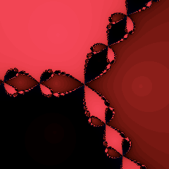
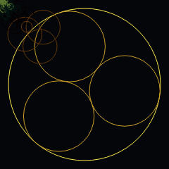
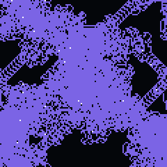
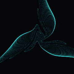
INDEX OF PLATES

The whole atlas as text — discoverer, definition, provenance and licence standing for every specimen. Each entry opens its live plate. This page is generated from the same array the atlas renders, so it cannot drift from the plates. 33 plates carry a HOUDINI · VEX port — the same published mathematics written for a Detail Wrangle, cooked and verified in Houdini before it shipped.

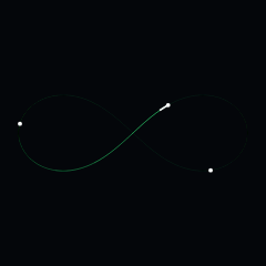
PL. 01

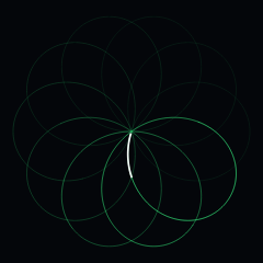
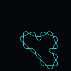
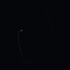
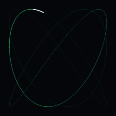
Lissajous Figure

CURVES / PARAMETRIC / STANDING WAVE

Nathaniel Bowditch, 1815 · Jules Lissajous, 1857

x(u) = A·sin(a·u + δ)
y(u) = B·sin(b·u)

Two perpendicular sinusoids plotted against each other. When a and b are small whole-number ratios the path closes into a standing knot; irrational ratios never close and fill the box. Bowditch found them with a compound pendulum forty years before Lissajous found them with mirrors and a tuning fork.

Origin — Bowditch (1815), independently Lissajous (1857)
Standing — Public domain — 19th-century mathematics
Constants — δ animates continuously; a and b set the ratio
HOUDINI · VEX — paste into a Detail Wrangle
// FORMA — PL. 01 · LISSAJOUS FIGURE — Nathaniel Bowditch, 1815 · Jules Lissajous, 1857
//   x(u) = A·sin(a·u + δ)
//   y(u) = B·sin(b·u)
// Paste into a Detail Wrangle (Run Over: Detail), no inputs needed.
// Written from the published mathematics, not adapted from any code.
// Defaults are the published values; comments give the measured live range.
// https://forma-gen.com/#plate=lissajous

float p_a     = 3;         // 1 .. 12  · a — horizontal frequency
float p_b     = 4;         // 1 .. 12  · b — vertical frequency
float p_delta = 0.6;       // 0 .. 3.14  · δ — phase offset

// The plate's own colour: FORMA's CURVES accent as a cosine ramp,
// brightest near t = 0 and t = 1, near-black around t = 0.5.
vector forma_ramp(float t){
  return set(
    0.11 + 0.1196 * cos(6.28318530718 * (t + 0)),
    0.46 + 0.5 * cos(6.28318530718 * (t + 0.05)),
    0.2453 + 0.2667 * cos(6.28318530718 * (t + 0.1)));
}

// One closed period of the figure: u over 2π at unit amplitude. Integer
// frequencies close the curve; the phase δ tilts it out of degeneracy.
int forma_n = 1600;

float TAU = 6.28318530718;
int prim = addprim(0, "polyline");
for (int i = 0; i <= forma_n; i++){
    float u = float(i) / float(forma_n) * TAU;
    // canvas y runs down; negated so the figure sits as the plate shows it
    int pt = addpoint(0, set(sin(p_a * u + p_delta), -sin(p_b * u), 0.0));
    // colour sweeps the bright lobe of the ramp along the curve
    float uu = float(i) / float(forma_n);
    setpointattrib(0, "Cd", pt, forma_ramp(0.8 + 0.3 * uu));
    addvertex(0, prim, pt);
}
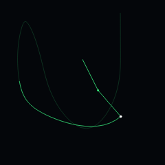
PL. 02

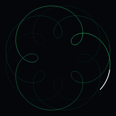
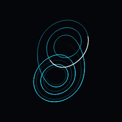
Rhodonea

CURVES / POLAR / SINUSOID

Guido Grandi, c. 1723

r(θ) = cos(k·θ),  k = n/d

A sinusoid in polar coordinates. Grandi named these rose curves for the obvious reason. When k is an integer the bloom has k petals if k is odd and 2k if it is even — a parity quirk that comes from whether the negative half of the cosine retraces the positive half or lands opposite it.

Origin — Guido Grandi, Italian mathematician, c. 1723
Standing — Public domain — 18th-century mathematics
Constants — n/d rational gives a closed curve; large d gives dense rosettes
HOUDINI · VEX — paste into a Detail Wrangle
// FORMA — PL. 02 · RHODONEA — Guido Grandi, c. 1723
//   r(θ) = cos(k·θ),  k = n/d
// Paste into a Detail Wrangle (Run Over: Detail), no inputs needed.
// Written from the published mathematics, not adapted from any code.
// Defaults are the published values; comments give the measured live range.
// https://forma-gen.com/#plate=rose

float p_n = 5;         // 1 .. 13  · n — numerator
float p_d = 4;         // 1 .. 13  · d — denominator

// The plate's own colour: FORMA's CURVES accent as a cosine ramp,
// brightest near t = 0 and t = 1, near-black around t = 0.5.
vector forma_ramp(float t){
  return set(
    0.11 + 0.1196 * cos(6.28318530718 * (t + 0)),
    0.46 + 0.5 * cos(6.28318530718 * (t + 0.05)),
    0.2453 + 0.2667 * cos(6.28318530718 * (t + 0.1)));
}

// r = cos(k·θ) with k = n/d closes after d full turns of θ, tracing every
// petal exactly once — the same span the plate walks.
int forma_n = 4000;

int   nn = int(p_n), dd = int(p_d);
float k = float(nn) / float(dd);
float turns = 6.28318530718 * float(dd);
int prim = addprim(0, "polyline");
for (int i = 0; i <= forma_n; i++){
    float th = float(i) / float(forma_n) * turns;
    float r  = cos(k * th);
    // canvas y runs down; negated so the curve sits as the plate shows it
    int pt = addpoint(0, set(r * cos(th), -r * sin(th), 0.0));
    // colour sweeps the bright lobe of the ramp along the curve
    float u = float(i) / float(forma_n);
    setpointattrib(0, "Cd", pt, forma_ramp(0.8 + 0.3 * u));
    addvertex(0, prim, pt);
}
PL. 03

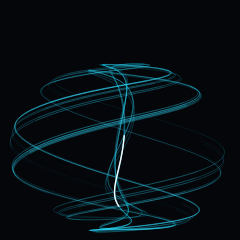
Epitrochoid

CURVES / ROULETTE / ROLLING CIRCLE

Albrecht Dürer, 1525 · Ptolemaic tradition

x(θ) = (R+r)·cos θ − h·cos(((R+r)/r)·θ)
y(θ) = (R+r)·sin θ − h·sin(((R+r)/r)·θ)

The path of a point fixed to a circle rolling around the outside of another circle. Dürer drew them by hand in 1525; the toy shop sells the hypotrochoid version as a Spirograph. Set h = r and you get the epicycloid, the curve the Ptolemaic astronomers used to explain retrograde motion.

Origin — Described by Dürer (1525); roulettes studied since antiquity
Standing — Public domain
Constants — Whole-number R/r closes the curve; h is the pen offset
HOUDINI · VEX — paste into a Detail Wrangle
// FORMA — PL. 03 · EPITROCHOID — Albrecht Dürer, 1525 · Ptolemaic tradition
//   x(θ) = (R+r)·cos θ − h·cos(((R+r)/r)·θ)
//   y(θ) = (R+r)·sin θ − h·sin(((R+r)/r)·θ)
// Paste into a Detail Wrangle (Run Over: Detail), no inputs needed.
// Written from the published mathematics, not adapted from any code.
// Defaults are the published values; comments give the measured live range.
// https://forma-gen.com/#plate=epitrochoid

float p_R = 8;         // 1 .. 14  · R — fixed circle
float p_r = 3;         // 1 .. 14  · r — rolling circle
float p_h = 5;         // 1 .. 14  · h — pen offset

// The plate's own colour: FORMA's CURVES accent as a cosine ramp,
// brightest near t = 0 and t = 1, near-black around t = 0.5.
vector forma_ramp(float t){
  return set(
    0.11 + 0.1196 * cos(6.28318530718 * (t + 0)),
    0.46 + 0.5 * cos(6.28318530718 * (t + 0.05)),
    0.2453 + 0.2667 * cos(6.28318530718 * (t + 0.1)));
}

// The pen closes after r full turns of the rolling contact — θ spans 2π·r,
// tracing every loop of the figure once, as the plate does.
int forma_n = 5000;

float TAU = 6.28318530718;
int   rr = int(rint(p_r));
float ratio = (p_R + p_r) / p_r;
float turns = TAU * float(rr);
int prim = addprim(0, "polyline");
for (int i = 0; i <= forma_n; i++){
    float th = float(i) / float(forma_n) * turns;
    float x = (p_R + p_r) * cos(th) - p_h * cos(ratio * th);
    float y = (p_R + p_r) * sin(th) - p_h * sin(ratio * th);
    // canvas y runs down; negated so the figure sits as the plate shows it
    int pt = addpoint(0, set(x, -y, 0.0));
    // colour sweeps the bright lobe of the ramp along the curve
    float u = float(i) / float(forma_n);
    setpointattrib(0, "Cd", pt, forma_ramp(0.8 + 0.3 * u));
    addvertex(0, prim, pt);
}
PL. 04

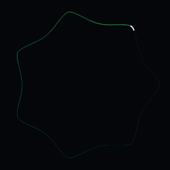
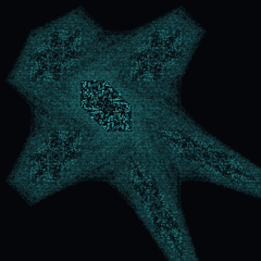
Superformula

CURVES / POLAR / SUPERELLIPSE

Johan Gielis, 2003

r(φ) = ( |cos(mφ/4)/a|^n₂ + |sin(mφ/4)/b|^n₃ )^(−1/n₁)

A generalisation of the superellipse that Gielis proposed as a single equation behind starfish, diatoms, flowers and shells. Four constants take it from circle to polygon to bloom. It is the one entry here with a genuine legal history: Gielis patented pattern synthesis using the operator, and the patent was enforced aggressively enough that it shadowed a well-known video game.

Origin — Johan Gielis, American Journal of Botany 90(3), 2003
Patent — EP1177529 / US7620527 — expired 10 May 2020
Standing — Free to use. The patent lapsed; formulas are not copyrightable.
HOUDINI · VEX — paste into a Detail Wrangle
// FORMA — PL. 04 · SUPERFORMULA — Johan Gielis, 2003
//   r(φ) = ( |cos(mφ/4)/a|^n₂ + |sin(mφ/4)/b|^n₃ )^(−1/n₁)
// Paste into a Detail Wrangle (Run Over: Detail), no inputs needed.
// Written from the published mathematics, not adapted from any code.
// Defaults are the published values; comments give the measured live range.
// https://forma-gen.com/#plate=superformula

float p_m  = 7;         // 1 .. 20  · m — rotational symmetry
float p_n1 = 0.6;       // 0.2 .. 8  · n₁
float p_n2 = 1.7;       // 0.2 .. 8  · n₂
float p_n3 = 1.7;       // 0.2 .. 8  · n₃
float p_a  = 1;         // 0.2 .. 3  · a — first semi-axis
float p_b  = 1;         // 0.2 .. 3  · b — second semi-axis

// The plate's own colour: FORMA's CURVES accent as a cosine ramp,
// brightest near t = 0 and t = 1, near-black around t = 0.5.
vector forma_ramp(float t){
  return set(
    0.11 + 0.1196 * cos(6.28318530718 * (t + 0)),
    0.46 + 0.5 * cos(6.28318530718 * (t + 0.05)),
    0.2453 + 0.2667 * cos(6.28318530718 * (t + 0.1)));
}

// Gielis's operator in polar form, one closed sweep of φ. a and b are the
// semi-axes the published operator divides by; unequal values are where the
// stretched starfish and diatom forms live. A non-finite r (n₁ near zero at
// a cusp) plots as the origin, exactly as the plate treats it.
int forma_n = 2400;

float TAU = 6.28318530718;
int prim = addprim(0, "polyline");
for (int i = 0; i <= forma_n; i++){
    float phi = float(i) / float(forma_n) * TAU;
    float ta = pow(abs(cos(p_m * phi / 4.0) / p_a), p_n2);
    float tb = pow(abs(sin(p_m * phi / 4.0) / p_b), p_n3);
    float r = pow(ta + tb, -1.0 / p_n1);
    if (!isfinite(r)) r = 0.0;
    // canvas y runs down; negated so the figure sits as the plate shows it
    int pt = addpoint(0, set(r * cos(phi), -r * sin(phi), 0.0));
    // colour sweeps the bright lobe of the ramp along the curve
    float u = float(i) / float(forma_n);
    setpointattrib(0, "Cd", pt, forma_ramp(0.8 + 0.3 * u));
    addvertex(0, prim, pt);
}
PL. 05

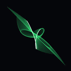
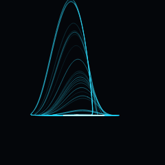
Harmonograph

CURVES / DAMPED / PENDULUM PAIR

Hugh Blackburn, 1844

x(t) = Σ Aᵢ·sin(fᵢ·t + φᵢ)·e^(−dᵢ·t)
y(t) = Σ Aⱼ·sin(fⱼ·t + φⱼ)·e^(−dⱼ·t)

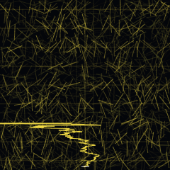
A Victorian drawing machine: two or three pendulums swinging on perpendicular axes, a pen on the last one. The exponential term is friction. What makes the figures beautiful is that the decay tightens the envelope while the phase keeps drifting, so the curve never quite retraces itself.

Origin — Hugh Blackburn, Glasgow, 1844
Standing — Public domain — a physical instrument, described openly
Constants — Frequencies near-but-not-equal give the slow beat
HOUDINI · VEX — paste into a Detail Wrangle
// FORMA — PL. 05 · HARMONOGRAPH — Hugh Blackburn, 1844
//   x(t) = Σ Aᵢ·sin(fᵢ·t + φᵢ)·e^(−dᵢ·t)
//   y(t) = Σ Aⱼ·sin(fⱼ·t + φⱼ)·e^(−dⱼ·t)
// Paste into a Detail Wrangle (Run Over: Detail), no inputs needed.
// Written from the published mathematics, not adapted from any code.
// Defaults are the published values; comments give the measured live range.
// https://forma-gen.com/#plate=harmonograph

float p_f1 = 2.01;      // 1 .. 8  · f₁
float p_f2 = 3;         // 1 .. 8  · f₂
float p_f3 = 3.01;      // 1 .. 8  · f₃
float p_f4 = 2;         // 1 .. 8  · f₄
float p_d  = 0.006;     // 0.001 .. 0.03  · damping

// The plate's own colour: FORMA's CURVES accent as a cosine ramp,
// brightest near t = 0 and t = 1, near-black around t = 0.5.
vector forma_ramp(float t){
  return set(
    0.11 + 0.1196 * cos(6.28318530718 * (t + 0)),
    0.46 + 0.5 * cos(6.28318530718 * (t + 0.05)),
    0.2453 + 0.2667 * cos(6.28318530718 * (t + 0.1)));
}

// Two damped sines per axis at unit amplitude, the second pendulum damped
// 1.4× harder — the plate's own ratio. The path is open: a harmonograph
// spirals inward as the pendulums die, it never closes.
int   forma_n  = 12000;
float forma_dt = 0.06;

int prim = addprim(0, "polyline");
for (int i = 0; i < forma_n; i++){
    float u  = float(i) * forma_dt;
    float e1 = exp(-p_d * u);
    float e2 = exp(-p_d * 1.4 * u);
    float x = sin(p_f1 * u) * e1 + sin(p_f2 * u) * e2;
    float y = sin(p_f3 * u) * e1 + sin(p_f4 * u) * e2;
    // canvas y runs down; negated so the figure sits as the plate shows it
    int pt = addpoint(0, set(x, -y, 0.0));
    // colour sweeps the bright lobe of the ramp along the path
    float uu = float(i) / float(forma_n);
    setpointattrib(0, "Cd", pt, forma_ramp(0.8 + 0.3 * uu));
    addvertex(0, prim, pt);
}
PL. 06

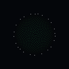
Phyllotaxis

CURVES / PACKING / GOLDEN ANGLE

Helmut Vogel, 1979 · after Kepler and Bravais

θ(n) = n · 137.508°
r(n) = c · nᵏ,  k = ½ for equal area

The arrangement of florets in a sunflower head. The angle is the golden angle, 360°(2−φ), and it is the unique rotation that never lets successive points line up into rows — which is exactly what a plant wants if every seed is to get light. Change it by a fifth of a degree and the spirals collapse into spokes.

Origin — Vogel's model, Mathematical Biosciences 44, 1979
Standing — Public domain — a description of a natural arrangement
Constants — 137.508° is the golden angle; c only sets the scale
HOUDINI · VEX — paste into a Detail Wrangle
// FORMA — PL. 06 · PHYLLOTAXIS — Helmut Vogel, 1979 · after Kepler and Bravais
//   θ(n) = n · 137.508°
//   r(n) = c · nᵏ,  k = ½ for equal area
// Paste into a Detail Wrangle (Run Over: Detail), no inputs needed.
// Written from the published mathematics, not adapted from any code.
// Defaults are the published values; comments give the measured live range.
// https://forma-gen.com/#plate=phyllotaxis

float p_angle = 137.508;   // 137 .. 138  · divergence angle (°)
float p_n     = 1400;      // 200 .. 3000  · floret count
float p_expo  = 0.5;       // 0.3 .. 0.8  · k — radial exponent

// The plate's own colour: FORMA's CURVES accent as a cosine ramp,
// brightest near t = 0 and t = 1, near-black around t = 0.5.
vector forma_ramp(float t){
  return set(
    0.11 + 0.1196 * cos(6.28318530718 * (t + 0)),
    0.46 + 0.5 * cos(6.28318530718 * (t + 0.05)),
    0.2453 + 0.2667 * cos(6.28318530718 * (t + 0.1)));
}

// Vogel's spiral as a point cloud: floret i sits at angle i·137.508° and
// radius (i/n)^k, so the disc fills the unit circle. k = ½ is the equal-area
// packing; below it the florets crowd the rim, above it the centre — the
// whole disc restructures. pscale mirrors the plate's growing floret size.
int nf = int(p_n);
float ga = radians(p_angle);
for (int i = 1; i <= nf; i++){
    float u  = float(i) / float(nf);
    float th = float(i) * ga;
    float r  = pow(u, p_expo);
    // canvas y runs down; negated so the spiral winds as the plate shows it
    int pt = addpoint(0, set(r * cos(th), -r * sin(th), 0.0));
    // the full ramp, as the plate sweeps it — the dark mid-radius ring is
    // the palette's own trough reading as contour on a dense disc
    setpointattrib(0, "Cd", pt, forma_ramp(u));
    setpointattrib(0, "pscale", pt, (0.6 + 1.6 * u) / 150.0);
}
PL. 07

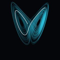
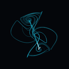
Lorenz Attractor

ATTRACTORS / FLOW / DIFFERENTIAL

Edward Lorenz, 1963

ẋ = σ(y − x)
ẏ = x(ρ − z) − y
ż = xy − βz

Lorenz was running a truncated weather model, restarted it from a rounded printout, and got a completely different forecast. The butterfly shape is the set the trajectory settles onto — bounded, never repeating, never crossing itself. This is the origin of the phrase "sensitive dependence on initial conditions".

Origin — E. N. Lorenz, "Deterministic Nonperiodic Flow", J. Atmos. Sci. 20, 1963
Standing — Public domain — a system of differential equations
Constants — σ=10, ρ=28, β=8/3 is the classic parameter set
HOUDINI · VEX — paste into a Detail Wrangle
// FORMA — PL. 07 · LORENZ ATTRACTOR — Edward Lorenz, 1963
//   ẋ = σ(y − x)
//   ẏ = x(ρ − z) − y
//   ż = xy − βz
// Paste into a Detail Wrangle (Run Over: Detail), no inputs needed.
// Written from the published mathematics, not adapted from any code.
// Defaults are the published values; comments give the measured live range.
// https://forma-gen.com/#plate=lorenz

float p_sigma = 10;        // 4 .. 20  · σ — Prandtl
float p_rho   = 28;        // 14 .. 60  · ρ — Rayleigh
float p_beta  = 2.667;     // 0.5 .. 5  · β — geometry

// The plate's own colour: FORMA's ATTRACTORS accent as a cosine ramp,
// brightest near t = 0 and t = 1, near-black around t = 0.5.
vector forma_ramp(float t){
  return set(
    0.0956 + 0.1039 * cos(6.28318530718 * (t + 0)),
    0.4041 + 0.4392 * cos(6.28318530718 * (t + 0.05)),
    0.46 + 0.5 * cos(6.28318530718 * (t + 0.1)));
}

// Euler integration matching the plate: dt = 0.005, 18000 steps, the first
// 400 discarded — the walk toward the attractor is not the attractor.
int   forma_steps = 18000;
int   forma_skip  = 400;
float forma_dt    = 0.005;

// Lorenz's z is conventionally the vertical; mapped onto Houdini's y-up.
float x = 0.1, y = 0.0, z = 0.0;
int prim = addprim(0, "polyline");
for (int i = 0; i < forma_steps; i++){
    float dx = p_sigma * (y - x);
    float dy = x * (p_rho - z) - y;
    float dz = x * y - p_beta * z;
    x += dx * forma_dt;  y += dy * forma_dt;  z += dz * forma_dt;
    if (i <= forma_skip) continue;
    int pt = addpoint(0, set(x, z, y));
    // colour sweeps the bright lobe of the ramp along the path
    float u = float(i - forma_skip) / float(forma_steps - forma_skip);
    setpointattrib(0, "Cd", pt, forma_ramp(0.8 + 0.3 * u));
    addvertex(0, prim, pt);
}
PL. 08

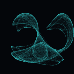
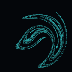
De Jong Map

ATTRACTORS / MAP / ITERATED

Peter de Jong, popularised 1980s

xₙ₊₁ = sin(a·yₙ) − cos(b·xₙ)
yₙ₊₁ = sin(c·xₙ) − cos(d·yₙ)

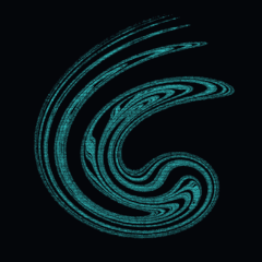
Four constants, two lines, and an unreasonable amount of structure. Plotted as a density histogram over a few hundred thousand iterations, the map produces veils and caustics that look photographed rather than computed. Almost every parameter set gives something; a few give something extraordinary.

Origin — Attributed to Peter de Jong; circulated via Scientific American
Standing — Public domain — an iterated map
Constants — Sweep any one constant slowly and the whole figure breathes
HOUDINI · VEX — paste into a Detail Wrangle
// FORMA — PL. 08 · DE JONG MAP — Peter de Jong, popularised 1980s
//   xₙ₊₁ = sin(a·yₙ) − cos(b·xₙ)
//   yₙ₊₁ = sin(c·xₙ) − cos(d·yₙ)
// Paste into a Detail Wrangle (Run Over: Detail), no inputs needed.
// Written from the published mathematics, not adapted from any code.
// Defaults are the published values; comments give the measured live range.
// https://forma-gen.com/#plate=dejong

float p_a = 1.641;     // -3 .. 3  · a
float p_b = 1.902;     // -3 .. 3  · b
float p_c = 0.316;     // -3 .. 3  · c
float p_d = 1.525;     // -3 .. 3  · d

// The plate's own colour: FORMA's ATTRACTORS accent as a cosine ramp,
// brightest near t = 0 and t = 1, near-black around t = 0.5.
vector forma_ramp(float t){
  return set(
    0.0956 + 0.1039 * cos(6.28318530718 * (t + 0)),
    0.4041 + 0.4392 * cos(6.28318530718 * (t + 0.05)),
    0.46 + 0.5 * cos(6.28318530718 * (t + 0.1)));
}

// The exposure replayed as a point cloud: iterate from (0.1, 0.1) and discard
// the first 20 landings, as the plate's expose() does — the walk toward the
// attractor is not the attractor.
int forma_pts  = 120000;
int forma_skip = 20;

float x = 0.1, y = 0.1;
for (int i = 0; i < forma_pts + forma_skip; i++){
    float nx = sin(p_a * y) - cos(p_b * x);
    float ny = sin(p_c * x) - cos(p_d * y);
    x = nx;  y = ny;
    if (i < forma_skip) continue;
    // canvas y runs down; negated so the figure sits as the plate shows it
    int pt = addpoint(0, set(x, -y, 0.0));
    // colour sweeps the bright lobe of the ramp across the exposure
    float u = float(i) / float(forma_pts + forma_skip);
    setpointattrib(0, "Cd", pt, forma_ramp(0.8 + 0.3 * u));
}
PL. 09

Clifford Map

ATTRACTORS / MAP / ITERATED

Clifford A. Pickover

xₙ₊₁ = sin(a·yₙ) + c·cos(a·xₙ)
yₙ₊₁ = sin(b·xₙ) + d·cos(b·yₙ)

A sibling of the de Jong map with the cosine terms scaled rather than subtracted. The result tends toward smoke and ribbon rather than veil. Pickover catalogued dozens of these in the late 1980s while looking for what he called "biomorphs".

Origin — Clifford A. Pickover, from his work on iterated maps
Standing — Public domain — an iterated map
Constants — Keep |c| and |d| near 1 for the densest structure
HOUDINI · VEX — paste into a Detail Wrangle
// FORMA — PL. 09 · CLIFFORD MAP — Clifford A. Pickover
//   xₙ₊₁ = sin(a·yₙ) + c·cos(a·xₙ)
//   yₙ₊₁ = sin(b·xₙ) + d·cos(b·yₙ)
// Paste into a Detail Wrangle (Run Over: Detail), no inputs needed.
// Written from the published mathematics, not adapted from any code.
// Defaults are the published values; comments give the measured live range.
// https://forma-gen.com/#plate=clifford

float p_a = -1.4;      // -3 .. 3  · a
float p_b = 1.6;       // -3 .. 3  · b
float p_c = 1;         // -2 .. 2  · c
float p_d = 0.7;       // -2 .. 2  · d

// The plate's own colour: FORMA's ATTRACTORS accent as a cosine ramp,
// brightest near t = 0 and t = 1, near-black around t = 0.5.
vector forma_ramp(float t){
  return set(
    0.0956 + 0.1039 * cos(6.28318530718 * (t + 0)),
    0.4041 + 0.4392 * cos(6.28318530718 * (t + 0.05)),
    0.46 + 0.5 * cos(6.28318530718 * (t + 0.1)));
}

// The exposure replayed as a point cloud: iterate from (0.1, 0.1) and discard
// the first 20 landings, as the plate's expose() does.
int forma_pts  = 120000;
int forma_skip = 20;

float x = 0.1, y = 0.1;
for (int i = 0; i < forma_pts + forma_skip; i++){
    float nx = sin(p_a * y) + p_c * cos(p_a * x);
    float ny = sin(p_b * x) + p_d * cos(p_b * y);
    x = nx;  y = ny;
    if (i < forma_skip) continue;
    // canvas y runs down; negated so the figure sits as the plate shows it
    int pt = addpoint(0, set(x, -y, 0.0));
    float u = float(i) / float(forma_pts + forma_skip);
    setpointattrib(0, "Cd", pt, forma_ramp(0.8 + 0.3 * u));
}
PL. 10

Thomas Attractor

ATTRACTORS / FLOW / CYCLIC SYMMETRY

René Thomas, 1999

ẋ = sin y − b·x
ẏ = sin z − b·y
ż = sin x − b·z

Cyclically symmetric in x, y and z — the same equation rotated through all three. Thomas described it as a particle drifting through a three-dimensional lattice of forces with friction b. Above b = 1 it dies to a point; below roughly 0.208 it becomes chaotic and starts wandering the lattice.

Origin — René Thomas, Int. J. Bifurcation and Chaos, 1999
Standing — Public domain — a system of differential equations
Constants — b ≈ 0.19 sits just inside the chaotic regime
HOUDINI · VEX — paste into a Detail Wrangle
// FORMA — PL. 10 · THOMAS ATTRACTOR — René Thomas, 1999
//   ẋ = sin y − b·x
//   ẏ = sin z − b·y
//   ż = sin x − b·z
// Paste into a Detail Wrangle (Run Over: Detail), no inputs needed.
// Written from the published mathematics, not adapted from any code.
// Defaults are the published values; comments give the measured live range.
// https://forma-gen.com/#plate=thomas

float p_b = 0.19;      // 0.05 .. 0.35  · b — dissipation

// The plate's own colour: FORMA's ATTRACTORS accent as a cosine ramp,
// brightest near t = 0 and t = 1, near-black around t = 0.5.
vector forma_ramp(float t){
  return set(
    0.0956 + 0.1039 * cos(6.28318530718 * (t + 0)),
    0.4041 + 0.4392 * cos(6.28318530718 * (t + 0.05)),
    0.46 + 0.5 * cos(6.28318530718 * (t + 0.1)));
}

// Euler integration matching the plate: dt = 0.02, 30000 steps from
// (1.1, 1.2, −0.6). Thomas is cyclically symmetric in x, y and z, so the
// axes carry over to Houdini's unchanged.
int   forma_steps = 30000;
float forma_dt    = 0.02;

float x = 1.1, y = 1.2, z = -0.6;
int prim = addprim(0, "polyline");
for (int i = 0; i < forma_steps; i++){
    float dx = sin(y) - p_b * x;
    float dy = sin(z) - p_b * y;
    float dz = sin(x) - p_b * z;
    x += dx * forma_dt;  y += dy * forma_dt;  z += dz * forma_dt;
    int pt = addpoint(0, set(x, y, z));
    // colour sweeps the bright lobe of the ramp along the path
    float u = float(i) / float(forma_steps);
    setpointattrib(0, "Cd", pt, forma_ramp(0.8 + 0.3 * u));
    addvertex(0, prim, pt);
}
PL. 11

Hénon Map

ATTRACTORS / MAP / QUADRATIC

Michel Hénon, 1976

xₙ₊₁ = 1 − a·xₙ² + yₙ
yₙ₊₁ = b·xₙ

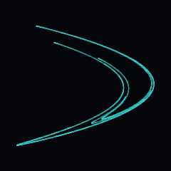
Hénon built this deliberately as the simplest possible map with a strange attractor — a stripped-down stand-in for a slice through the Lorenz system. Zoom into any part of the arc and you find it is not a line at all but a Cantor set of lines, all the way down.

Origin — M. Hénon, Comm. Math. Phys. 50, 1976
Standing — Public domain — an iterated map
Constants — a=1.4, b=0.3 is the canonical pair
HOUDINI · VEX — paste into a Detail Wrangle
// FORMA — PL. 11 · HÉNON MAP — Michel Hénon, 1976
//   xₙ₊₁ = 1 − a·xₙ² + yₙ
//   yₙ₊₁ = b·xₙ
// Paste into a Detail Wrangle (Run Over: Detail), no inputs needed.
// Written from the published mathematics, not adapted from any code.
// Defaults are the published values; comments give the measured live range.
// https://forma-gen.com/#plate=henon

float p_a = 1.4;       // 1 .. 1.42  · a
float p_b = 0.3;       // 0.1 .. 0.4  · b

// The plate's own colour: FORMA's ATTRACTORS accent as a cosine ramp,
// brightest near t = 0 and t = 1, near-black around t = 0.5.
vector forma_ramp(float t){
  return set(
    0.0956 + 0.1039 * cos(6.28318530718 * (t + 0)),
    0.4041 + 0.4392 * cos(6.28318530718 * (t + 0.05)),
    0.46 + 0.5 * cos(6.28318530718 * (t + 0.1)));
}

// The exposure replayed as a point cloud: iterate from (0.1, 0.1) and discard
// the first 20 landings, as the plate's expose() does. The attractor is a
// thin crescent — covering little of its box is its published shape.
int forma_pts  = 120000;
int forma_skip = 20;

float x = 0.1, y = 0.1;
for (int i = 0; i < forma_pts + forma_skip; i++){
    float nx = 1.0 - p_a * x * x + y;
    float ny = p_b * x;
    x = nx;  y = ny;
    if (i < forma_skip) continue;
    // canvas y runs down; negated so the figure sits as the plate shows it
    int pt = addpoint(0, set(x, -y, 0.0));
    float u = float(i) / float(forma_pts + forma_skip);
    setpointattrib(0, "Cd", pt, forma_ramp(0.8 + 0.3 * u));
}
PL. 12

Ikeda Map

ATTRACTORS / MAP / OPTICAL CAVITY

Kensuke Ikeda, 1979

tₙ = 0.4 − 6/(1 + xₙ² + yₙ²)
xₙ₊₁ = 1 + u(xₙ·cos tₙ − yₙ·sin tₙ)
yₙ₊₁ = u(xₙ·sin tₙ + yₙ·cos tₙ)

Derived from light circulating in a ring cavity filled with a nonlinear medium — the rotation angle depends on the intensity, so bright parts of the beam twist further than dim ones. The attractor is a spiral shell that keeps folding back into itself. Chaotic above u ≈ 0.6, and only transiently past u ≈ 0.9 — there the orbit wanders the shell for a while, then falls onto a stable fixed point far outside it.

Origin — K. Ikeda, Optics Communications 30, 1979
Standing — Public domain — a physical model published openly
Constants — u = 0.9 is the classic choice; the attractor dies in a crisis near u ≈ 0.902, so the slider stops at 0.9
HOUDINI · VEX — paste into a Detail Wrangle
// FORMA — PL. 12 · IKEDA MAP — Kensuke Ikeda, 1979
//   tₙ = 0.4 − 6/(1 + xₙ² + yₙ²)
//   xₙ₊₁ = 1 + u(xₙ·cos tₙ − yₙ·sin tₙ)
//   yₙ₊₁ = u(xₙ·sin tₙ + yₙ·cos tₙ)
// Paste into a Detail Wrangle (Run Over: Detail), no inputs needed.
// Written from the published mathematics, not adapted from any code.
// Defaults are the published values; comments give the measured live range.
// https://forma-gen.com/#plate=ikeda

float p_u = 0.9;       // 0.6 .. 0.9  · u — dissipation

// The plate's own colour: FORMA's ATTRACTORS accent as a cosine ramp,
// brightest near t = 0 and t = 1, near-black around t = 0.5.
vector forma_ramp(float t){
  return set(
    0.0956 + 0.1039 * cos(6.28318530718 * (t + 0)),
    0.4041 + 0.4392 * cos(6.28318530718 * (t + 0.05)),
    0.46 + 0.5 * cos(6.28318530718 * (t + 0.1)));
}

// The exposure replayed as a point cloud: iterate from (0.1, 0.1) and discard
// the first 20 landings, as the plate's expose() does.
int forma_pts  = 120000;
int forma_skip = 20;

float x = 0.1, y = 0.1;
for (int i = 0; i < forma_pts + forma_skip; i++){
    float tn = 0.4 - 6.0 / (1.0 + x * x + y * y);
    float nx = 1.0 + p_u * (x * cos(tn) - y * sin(tn));
    float ny = p_u * (x * sin(tn) + y * cos(tn));
    x = nx;  y = ny;
    if (i < forma_skip) continue;
    // canvas y runs down; negated so the figure sits as the plate shows it
    int pt = addpoint(0, set(x, -y, 0.0));
    float u = float(i) / float(forma_pts + forma_skip);
    setpointattrib(0, "Cd", pt, forma_ramp(0.8 + 0.3 * u));
}
PL. 13

Mandelbrot Set

FRACTALS / ESCAPE TIME / QUADRATIC

Benoît Mandelbrot, 1980 · after Fatou and Julia

zₙ₊₁ = zₙ² + c,  z₀ = 0
c ∈ M  ⟺  |zₙ| stays bounded

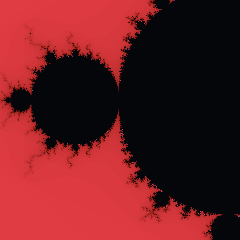
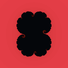
The set of complex c for which the orbit of zero never escapes. Its boundary is where all the detail lives — infinitely long, everywhere rough, and containing distorted copies of the whole set at every scale. Colour here is escape time, not membership: the interior is genuinely black.

Origin — Named for Mandelbrot (1980); built on Fatou and Julia, 1917–19
Standing — Public domain — a set defined by an iteration
Constants — Iteration ceiling trades detail for speed
PL. 14

Julia Set

FRACTALS / ESCAPE TIME / FIXED C

Gaston Julia, 1918 · Pierre Fatou, 1917

zₙ₊₁ = zₙ² + c,  z₀ = pixel
c = μ/2 − μ²/4,  μ = |μ|·e^(iθ)

The same iteration as the Mandelbrot set with the roles swapped: c is fixed and the starting point varies. Every c gives a different Julia set, and the Mandelbrot set is precisely the map of which ones are connected. Julia worked all of this out without ever seeing one drawn.

Origin — Gaston Julia, Journal de Mathématiques Pures et Appliquées, 1918
Standing — Public domain — a century old
Constants — |μ| under 1 keeps c inside the main cardioid, so the set stays connected; over 1 breaks it into dust
PL. 15

Barnsley Fern

FRACTALS / IFS / AFFINE

Michael Barnsley, 1988

four affine maps fᵢ(x,y) = Aᵢ·(x,y)ᵀ + bᵢ
applied at random with fixed probabilities

An iterated function system: pick one of four affine transforms at random, apply it, plot the point, repeat. The attractor is the fern regardless of where you start. One map draws the stem, one the left fronds, one the right, and one — used 85% of the time — shrinks and rotates everything upward.

Origin — M. Barnsley, "Fractals Everywhere", 1988
Standing — The IFS coefficients are mathematical facts, not expression
Constants — The stem map fires 1% of the time
PL. 16

Chaos Game

FRACTALS / IFS / VERTEX JUMP

Michael Barnsley, 1988 · Sierpiński, 1915

pₙ₊₁ = pₙ + r·(vₖ − pₙ),  vₖ a random vertex

Mark some vertices, start anywhere, and repeatedly jump a fixed fraction of the way toward a randomly chosen one. With three vertices and r = ½ you get Sierpiński's triangle — a shape defined by removal, arrived at by pure accumulation. Other vertex counts and ratios give lattices nobody has bothered to name.

Origin — The game is Barnsley's; the triangle is Sierpiński, 1915
Standing — Public domain
Constants — r = 1/2 with 3 vertices is the classic; try 5 vertices at 0.63
PL. 17

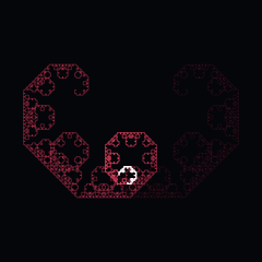
Heighway Dragon

FRACTALS / L-SYSTEM / PAPER FOLD

John Heighway, William Harter, Bruce Banks, 1966

fold a strip in half n times, unfold to 90°
turn sequence: Lₙ₊₁ = Lₙ · L · reverse(swap(Lₙ))

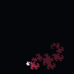
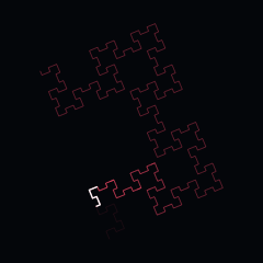
Fold a strip of paper in half repeatedly, then open every crease to a right angle. Three NASA physicists worked it out in 1966; Michael Crichton put it in the chapter headings of Jurassic Park. It tiles the plane with copies of itself and never crosses its own path.

Origin — Heighway, Harter and Banks at NASA, 1966
Standing — Public domain — a folding rule
Constants — Order above 16 exceeds what a plate this size can resolve
PL. 18

Hilbert Curve

FRACTALS / SPACE FILLING / RECURSIVE

David Hilbert, 1891

a bijection [0,1] → [0,1]²
built by recursive quadrant subdivision

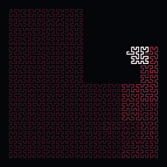
A line that visits every point of a square. Hilbert published it a year after Peano found the first such curve, and Hilbert's version has the useful property that points close together on the line stay close together in the square — which is why it is now used for image tiling, database indexing and heatmap layouts.

Origin — D. Hilbert, Mathematische Annalen 38, 1891
Standing — Public domain
Constants — Order n visits 4ⁿ cells
PL. 19

Fractional Brownian Motion

FIELDS / NOISE / OCTAVE SUM

Mandelbrot & Van Ness, 1968

fBm(p) = Σᵢ aⁱ · noise(2ⁱ·p),  a < 1

Octaves of the same noise summed at doubling frequency and halving amplitude. This is the single most load-bearing function in procedural graphics — terrain, cloud, marble, rust and smoke are all this with different post-processing. The exponent controls how rough the result feels.

Origin — Mandelbrot & Van Ness, SIAM Review 10, 1968
Standing — Public domain — a summation rule
Constants — Octaves above 8 stop being visible at screen resolution
PL. 20

Gradient Noise

FIELDS / NOISE / GRADIENT LATTICE

Ken Perlin, 1985

n(p) = interpolate over lattice corners of
       gᵢ · (p − cᵢ),  gᵢ pseudo-random unit vectors

Perlin built this for Tron and it won him an Academy Award. Unlike value noise, which interpolates random values, gradient noise interpolates random slopes — so the zero crossings land on the lattice and the result has no visible blockiness. His later simplex variant was patented; that patent expired in January 2022.

Origin — K. Perlin, "An Image Synthesizer", SIGGRAPH 1985
Patent — US6867776 covered the simplex construction — expired 8 Jan 2022
Standing — The 1985 gradient construction was never patented. Free.
PL. 21

Cellular Noise

FIELDS / NOISE / NEAREST FEATURE

Steven Worley, 1996

F₁(p) = min‖p − featureᵢ‖
F₂ − F₁ gives the cell borders

Scatter feature points, then colour every pixel by its distance to the nearest one. Worley published it as a texture basis function for stone, scale, leather and cracked mud. Taking the difference of the two nearest distances instead gives clean Voronoi edges, which is how most crystal and cell-wall shaders are built.

Origin — S. Worley, "A Cellular Texture Basis Function", SIGGRAPH 1996
Standing — Public domain — a distance function over scattered points
Constants — Jitter 0 collapses to a regular grid
PL. 22

Domain Warping

FIELDS / NOISE / INPUT TRANSFORM

A folk technique of procedural graphics

q = fbm(p)
r = fbm(p + 4q)
out = fbm(p + 4r)

Instead of transforming the output of a noise function, transform its input — with more noise. Two levels of this turn bland fBm into something that looks like marbled paper, nebulae or oil on water. The cost is only a few extra noise evaluations, which is why it appears in almost every serious shader library.

Origin — No single author; long-standing practice, documented widely
Standing — Public domain — function composition
Constants — Warp strength above ~6 dissolves the structure entirely
PL. 23

Flow Field

FIELDS / ADVECTION / VECTOR FIELD

Standard practice; after Perlin's vector fields

θ(p) = 2π · fbm(p)
pₙ₊₁ = pₙ + s·(cos θ, sin θ)

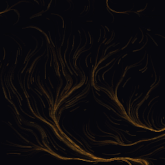
Read an angle out of a noise field at every point, then let particles drift along it leaving trails. The technique is the backbone of a whole genre of plotter art: the field is smooth, so neighbouring particles follow nearly the same path and the drawing organises itself into visible currents.

Origin — Common practice; the underlying idea is Perlin's vector noise
Standing — Public domain
Constants — Low turn scale gives laminar flow; high gives turbulence
PL. 24

Game of Life

AUTOMATA / AUTOMATON / 2D TOTALISTIC

John Horton Conway, 1970

live cell with 2 or 3 live neighbours survives
dead cell with exactly 3 live neighbours is born

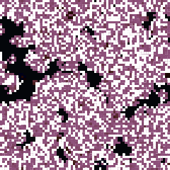
Two rules on a square grid, and the result is Turing complete. Conway wanted the simplest set of rules where neither explosive growth nor extinction was obvious, and he found it by hand with a Go board. He came to resent how thoroughly it overshadowed the rest of his mathematics.

Origin — J. H. Conway, 1970; popularised by Martin Gardner in Scientific American
Standing — Public domain — two transition rules
Constants — Initial density near 0.3 gives the longest-lived soups
PL. 25

Rule 30

AUTOMATA / AUTOMATON / 1D ELEMENTARY

Stephen Wolfram, 1983

aᵢ′ = aᵢ₋₁ XOR (aᵢ OR aᵢ₊₁)

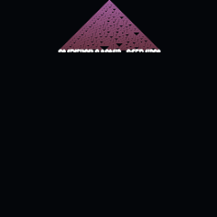
A one-dimensional automaton, one line of cells, each new row derived from the one above by looking at three neighbours. From a single black cell it produces a pattern with a provably random-looking centre column — random enough that Mathematica used it as a pseudo-random generator for years. Nobody has proved it never repeats.

Origin — S. Wolfram, "Statistical Mechanics of Cellular Automata", 1983
Standing — The rule is public domain. Wolfram's book text is not; his rules are.
Constants — Rule number 0–255 selects one of the 256 elementary automata
PL. 26

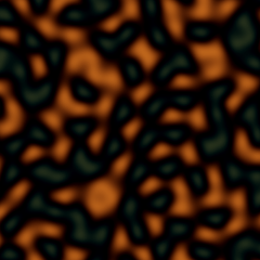
Gray–Scott Reaction–Diffusion

AUTOMATA / PDE / REACTION DIFFUSION

Peter Gray & Stephen Scott, 1983 · after Turing, 1952

∂u/∂t = Dᵤ∇²u − uv² + f(1−u)
∂v/∂t = D᷅∇²v + uv² − (f+k)v

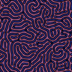
Two chemicals: one fed in, one that consumes it autocatalytically and decays. Turing predicted in 1952 that such a system could break its own symmetry and produce stripes and spots, which is where animal coats come from. The feed and kill rates decide whether you get coral, mitosis, worms or a slow death.

Origin — Gray & Scott, Chem. Eng. Sci., 1983; Turing, Phil. Trans. R. Soc. B, 1952
Standing — Public domain — a pair of partial differential equations
Constants — f=0.037 k=0.06 gives coral; f=0.029 k=0.057 gives mitosis. The lattice sets the pattern scale, not just the detail — more cells means more, smaller features
PL. 27

Diffusion-Limited Aggregation

AUTOMATA / GROWTH / RANDOM WALK

Thomas Witten & Leonard Sander, 1981

release a random walker; when it touches
the cluster, it sticks there permanently

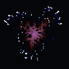
Particles wander at random until they bump into a growing cluster, then freeze. Because the outer tips intercept walkers before they can reach the interior, the result is always branched and never solid. This is the shape of electrodeposition, dielectric breakdown, mineral dendrites and lightning.

Origin — T. A. Witten & L. M. Sander, Phys. Rev. Lett. 47, 1981
Standing — Public domain — a growth process
Constants — Sticking probability below 1 thickens the branches
PL. 28

Truchet Tiles

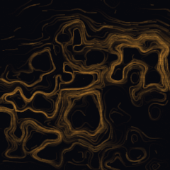
LATTICES / TILING / ROTATION SET

Sébastien Truchet, 1704

each cell takes one of k rotations,
chosen by a hash of its coordinates

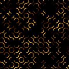
Father Truchet, a Dominican priest, catalogued what happens when you tile a plane with a single square split diagonally and let each tile take any of four rotations. The quarter-arc variant — two arcs joining opposite midpoints — produces continuous meandering loops that never terminate.

Origin — Sébastien Truchet, Mémoires de l'Académie Royale, 1704
Standing — Public domain — three centuries old
Constants — Arc weight near 0.16 of cell width reads best
PL. 29

Voronoi Diagram

LATTICES / PARTITION / NEAREST SITE

Georgy Voronoy, 1908 · Descartes, 1644

cell(sᵢ) = { p : ‖p − sᵢ‖ ≤ ‖p − sⱼ‖ ∀j }

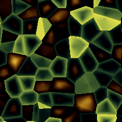
Divide the plane so every point belongs to whichever site is nearest. Descartes sketched the idea for the distribution of matter in the solar system; Voronoy formalised it. It is the dual of the Delaunay triangulation and shows up wherever territory is decided by proximity — cell walls, crystal grains, service areas, giraffe coats.

Origin — G. Voronoy, 1908; anticipated by Descartes (1644) and Dirichlet
Standing — Public domain
Constants — Sites drift on slow circular orbits here
PL. 30

Circle Packing

LATTICES / PACKING / GREEDY GROWTH

Classical; the greedy method is folklore

place a candidate at random;
grow its radius until it meets another or the edge

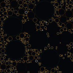
The naive algorithm — propose a centre, expand until something stops it, keep it if it is big enough — is not optimal packing in any mathematical sense, but it is the one that makes the drawings. Density falls off predictably, which is why the plate always ends up with a few large discs and a fine gravel of small ones.

Origin — Circle packing is classical; this greedy variant is common practice
Standing — Public domain
Constants — Attempts per frame governs how fine the gravel gets
PL. 31

Ulam Spiral

LATTICES / NUMBER THEORY / SPIRAL

Stanisław Ulam, 1963

walk the integers outward in a square spiral;
mark n when n is prime

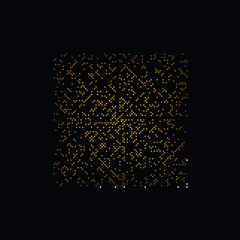
Ulam drew this while bored in a meeting. Write the whole numbers in a spiral and mark the primes: they fall on diagonals rather than scattering. Those diagonals correspond to prime-rich quadratic polynomials, and why some quadratics are so much richer than others is still open.

Origin — S. Ulam, 1963; published by Gardner in Scientific American, 1964
Standing — Public domain — an observation about integers
Constants — Larger extents make the diagonal structure clearer
PL. 32

Cosine Gradient

COLOUR / GRADIENT / COSINE BASIS

Formulated by Inigo Quilez

colour(t) = a + b · cos( 2π · (c·t + d) )
with a, b, c, d ∈ ℝ³

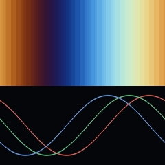
Twelve numbers describe an entire gradient. Each channel is its own cosine, so shifting d rotates the hue relationship without touching the brightness envelope. It is far more compact than a stop list and, unlike one, it is trivially differentiable — which matters if you are feeding it into a shader.

Origin — Formulated and published openly by Inigo Quilez
Standing — A formula, freely published. Credit given as a matter of courtesy.
Constants — a = offset, b = amplitude, c = frequency, d = phase
PL. 33

Easing Curves

COLOUR / INTERPOLATION / POLYNOMIAL

Robert Penner, 2001 · the polynomials are older

quad  f(t) = t²
cubic f(t) = t³
sine  f(t) = 1 − cos(πt/2)
expo  f(t) = 2^(10(t−1))

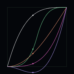
The interpolation curves that make motion read as physical rather than mechanical. Penner catalogued and named them for Flash designers in 2001; the underlying functions are just polynomials and trigonometry, some of them centuries old. The names stuck so thoroughly that they are now effectively an interface standard.

Origin — Named set popularised by Robert Penner, 2001
Standing — The functions are elementary mathematics — public domain
Constants — Every curve here passes through (0,0) and (1,1)
PL. 34

Burning Ship Fractal

FRACTALS / ESCAPE TIME / NON-ANALYTIC

Michael Michelitsch & Otto E. Rössler, 1992

z_{n+1} = (|Re(z_n)| + i|Im(z_n)|)² + c

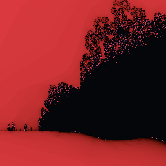
A variation of the Mandelbrot set where the absolute values of the real and imaginary components are taken before squaring at each iteration. The non-analytic transformation breaks Cauchy-Riemann symmetry, creating a fractal structure resembling a burning ship with intricate mast detail.

Origin — M. Michelitsch & O. E. Rössler, Computers & Graphics 16(4), 1992
Standing — Public domain — complex dynamical system
Constants — Iter governs calculation depth; cx/cy sets target coordinates
PL. 35

Newton Fractal

FRACTALS / ROOT FINDING / POLYNOMIAL

Sir Isaac Newton, 1669 · Arthur Cayley, 1879

z_{n+1} = z_n − (z_n³ − 1)/(3z_n²)

Newton's method for finding roots applied to the complex polynomial z³ − 1 = 0. Cayley asked in 1879 which starting points converge to which of the three roots of unity. The boundaries separating the basins of attraction are infinitely intricate fractals.

Origin — Sir Isaac Newton (1669), generalised by Arthur Cayley (1879)
Standing — Public domain — root-finding algorithm
Constants — Iter sets convergence limit; relax softens basin boundaries
PL. 36

Apollonian Gasket

LATTICES / CIRCLE PACKING / RECURSIVE

Apollonius of Perga, c. 200 BC · Frederick Soddy, 1936

(k₁ + k₂ + k₃ + k₄)² = 2(k₁² + k₂² + k₃² + k₄²)

Repeatedly filling the interstices between mutually tangent circles with smaller tangent circles. Apollonius posed the problem of circle tangency in antiquity; Soddy rediscovered the curvature formula in 1936 as the Kiss Precise poem. The resulting fractal limit set has a Hausdorff dimension of approximately 1.30568.

Origin — Apollonius of Perga (c. 200 BC), curvature theorem by Soddy (1936)
Standing — Public domain — ancient geometry theorem
Constants — Depth controls recursion level; spin animates rotation
PL. 37

Turmite Automaton

AUTOMATA / AUTOMATON / 2D TURING

A. K. Dewdney, 1989 · Greg Turk & Jim Propp, 1986

(state, color) → (new_color, turn, new_state)

A 2D Turing Machine that moves on a grid, changing the color of cells and turning relative to its orientation. Named by Dewdney as a pun on termite. Depending on the rule table, turmites produce chaotic highways, spiral growth, or structured periodic crystals.

Origin — Dewdney (1989), Turk & Propp (1986)
Standing — Public domain — cellular automaton model
Constants — Grid size sets canvas resolution; rule selects state transitions
PL. 38

Gumowski–Mira Map

ATTRACTORS / MAP / BEAM DYNAMICS

Igor Gumowski & Christian Mira, 1980

G(x) = μx + 2(1−μ)x²/(1+x²)
xₙ₊₁ = yₙ + α·yₙ(1 − σ·yₙ²) + G(xₙ)
yₙ₊₁ = −xₙ + G(xₙ₊₁)

Gumowski and Mira were modelling the transverse oscillation of particle beams in CERN’s storage rings when they found this recurrence. Each starting point traces its own chain of islands, and their superposition looks unreasonably biological — moths, jellyfish, orchids — for a map built from a single rational function. The small α term is a whisper of dissipation that slowly sharpens the figure.

Origin — I. Gumowski & C. Mira, "Recurrences and Discrete Dynamic Systems", Lecture Notes in Mathematics 809, Springer, 1980
Standing — Public domain — an iterated map
Constants — σ = 0.05 as published; μ selects the figure, and nearly every value draws a different one
HOUDINI · VEX — paste into a Detail Wrangle
// FORMA — PL. 38 · GUMOWSKI–MIRA MAP — Igor Gumowski & Christian Mira, 1980
//   G(x) = μx + 2(1−μ)x²/(1+x²)
//   xₙ₊₁ = yₙ + α·yₙ(1 − σ·yₙ²) + G(xₙ)
//   yₙ₊₁ = −xₙ + G(xₙ₊₁)
// Paste into a Detail Wrangle (Run Over: Detail), no inputs needed.
// Written from the published mathematics, not adapted from any code.
// Defaults are the published values; comments give the measured live range.
// https://forma-gen.com/#plate=mira

float p_m     = -0.496;    // -0.85 .. 0.35  · μ — nonlinearity
float p_a     = 0.008;     // 0 .. 0.02  · α — dissipation
float p_sigma = 0.05;      // 0 .. 0.12  · σ — cubic term
float p_run   = 700;       // 100 .. 3000  · orbit length per seed

// The plate's own colour: FORMA's ATTRACTORS accent as a cosine ramp,
// brightest near t = 0 and t = 1, near-black around t = 0.5.
vector forma_ramp(float t){
  return set(
    0.0956 + 0.1039 * cos(6.28318530718 * (t + 0)),
    0.4041 + 0.4392 * cos(6.28318530718 * (t + 0.05)),
    0.46 + 0.5 * cos(6.28318530718 * (t + 0.1)));
}

// Nearly conservative: each start owns its own island chain rather than
// falling onto one attractor, so the figure is many short orbits from
// scattered seeds superposed — which is what the published pictures are.
int forma_pts = 120000;

float x = 0.0, y = 0.0;
int   run = int(p_run) + 1, si = 0;   // force a seed on the first step
for (int i = 0; i < forma_pts; i++){
    if (++run > int(p_run)){
        run = 0;
        // deterministic scattered restarts, mirroring the plate's seeded rng
        float rad = 0.5 + 11.0 * random(si * 2);
        float th  = 6.28318530718 * random(si * 2 + 1);
        x = rad * cos(th);  y = rad * sin(th);
        si++;
    }
    float gx = p_m * x + 2.0 * (1.0 - p_m) * x * x / (1.0 + x * x);
    float nx = y + p_a * y * (1.0 - p_sigma * y * y) + gx;
    float gn = p_m * nx + 2.0 * (1.0 - p_m) * nx * nx / (1.0 + nx * nx);
    float ny = -x + gn;      // the old x — the map reads it before it moves
    x = nx;  y = ny;
    // canvas y runs down; negated so the figure sits as the plate shows it
    int pt = addpoint(0, set(x, -y, 0.0));
    float u = float(i) / float(forma_pts);
    setpointattrib(0, "Cd", pt, forma_ramp(0.8 + 0.3 * u));
}
PL. 39

Hopalong

ATTRACTORS / MAP / PIECEWISE ROOT

Barry Martin, 1986

xₙ₊₁ = yₙ − sign(xₙ)·√|b·xₙ − c|
yₙ₊₁ = a − xₙ

Martin’s orbit hops between interleaving rings, and the rings assemble into wallpaper. Dewdney printed it under the title "Wallpaper for the mind" and readers left it running for days. It never settles and never repeats — the pattern keeps growing outward for as long as the machine keeps iterating, which is why the exposure below restarts the orbit once it has filled its measured frame.

Origin — Barry Martin, Aston University; published in A. K. Dewdney’s "Computer Recreations", Scientific American, September 1986
Standing — Public domain — an iterated map
Constants — Almost any (a, b, c) makes wallpaper; the window is measured from the orbit itself
HOUDINI · VEX — paste into a Detail Wrangle
// FORMA — PL. 39 · HOPALONG — Barry Martin, 1986
//   xₙ₊₁ = yₙ − sign(xₙ)·√|b·xₙ − c|
//   yₙ₊₁ = a − xₙ
// Paste into a Detail Wrangle (Run Over: Detail), no inputs needed.
// Written from the published mathematics, not adapted from any code.
// Defaults are the published values; comments give the measured live range.
// https://forma-gen.com/#plate=hopalong

float p_a = 2;         // -10 .. 10  · a
float p_b = 1;         // 0.05 .. 3  · b
float p_c = 0;         // 0 .. 8  · c

// The plate's own colour: FORMA's ATTRACTORS accent as a cosine ramp,
// brightest near t = 0 and t = 1, near-black around t = 0.5.
vector forma_ramp(float t){
  return set(
    0.0956 + 0.1039 * cos(6.28318530718 * (t + 0)),
    0.4041 + 0.4392 * cos(6.28318530718 * (t + 0.05)),
    0.46 + 0.5 * cos(6.28318530718 * (t + 0.1)));
}

// The plate measures the orbit's extent to size its window, then replays the
// same orbit; geometry needs no window, so this is the orbit itself — one
// deterministic walk from the origin, growing ring by ring.
int forma_pts = 220000;

float x = 0.0, y = 0.0;
for (int i = 0; i < forma_pts; i++){
    float nx = y - sign(x) * sqrt(abs(p_b * x - p_c));
    y = p_a - x;
    x = nx;
    // canvas y runs down; negated so the figure sits as the plate shows it
    int pt = addpoint(0, set(x, -y, 0.0));
    float u = float(i) / float(forma_pts);
    setpointattrib(0, "Cd", pt, forma_ramp(0.8 + 0.3 * u));
}
PL. 40

Chirikov Standard Map

ATTRACTORS / MAP / KICKED ROTOR

Boris Chirikov, 1969

pₙ₊₁ = pₙ + K·sin θₙ  (mod 2π)
θₙ₊₁ = θₙ + pₙ₊₁  (mod 2π)

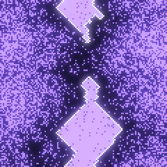
The phase portrait of a rotor kicked once per revolution, and the standard test problem of Hamiltonian chaos. Below the critical coupling, invariant circles wall the chaotic regions into bands; near K ≈ 0.9716 the last circle — the one with the golden-mean winding number — breaks, and orbits can finally diffuse across the whole cylinder. Islands draw themselves as rings, the chaotic sea as speckle.

Origin — B. V. Chirikov, preprint 267, Institute of Nuclear Physics, Novosibirsk, 1969; Physics Reports 52, 1979
Standing — Public domain — an area-preserving map
Constants — K ≈ 0.9716 is critical: the last invariant circle breaks there
HOUDINI · VEX — paste into a Detail Wrangle
// FORMA — PL. 40 · CHIRIKOV STANDARD MAP — Boris Chirikov, 1969
//   pₙ₊₁ = pₙ + K·sin θₙ  (mod 2π)
//   θₙ₊₁ = θₙ + pₙ₊₁  (mod 2π)
// Paste into a Detail Wrangle (Run Over: Detail), no inputs needed.
// Written from the published mathematics, not adapted from any code.
// Defaults are the published values; comments give the measured live range.
// https://forma-gen.com/#plate=standard

float p_K   = 0.972;     // 0.1 .. 2.6  · K — kick strength
float p_run = 400;       // 50 .. 2000  · orbit length per seed

// The plate's own colour: FORMA's ATTRACTORS accent as a cosine ramp,
// brightest near t = 0 and t = 1, near-black around t = 0.5.
vector forma_ramp(float t){
  return set(
    0.0956 + 0.1039 * cos(6.28318530718 * (t + 0)),
    0.4041 + 0.4392 * cos(6.28318530718 * (t + 0.05)),
    0.46 + 0.5 * cos(6.28318530718 * (t + 0.1)));
}

// Area-preserving, so there is no attractor to fall onto — every start keeps
// its own orbit forever. Short runs from scattered seeds are the honest
// rendering: islands close into rings, chaos arrives as speckle.
int forma_pts = 120000;

float TAU = 6.28318530718;
float th = 0.0, pn = 0.0;
int   run = int(p_run) + 1, si = 0;   // force a seed on the first step
for (int i = 0; i < forma_pts; i++){
    if (++run > int(p_run)){
        run = 0;
        // deterministic scattered restarts, mirroring the plate's seeded rng
        th = TAU * random(si * 2);
        pn = TAU * random(si * 2 + 1);
        si++;
    }
    pn = pn + p_K * sin(th);
    pn = pn - TAU * floor(pn / TAU);
    th = th + pn;
    th = th - TAU * floor(th / TAU);
    // canvas y runs down; flipped within the torus square to match the plate
    int pt = addpoint(0, set(th, TAU - pn, 0.0));
    float u = float(i) / float(forma_pts);
    setpointattrib(0, "Cd", pt, forma_ramp(0.8 + 0.3 * u));
}
PL. 41

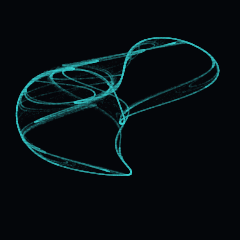
Rössler Attractor

ATTRACTORS / FLOW / FOLDED BAND

Otto Rössler, 1976

ẋ = −y − z
ẏ = x + a·y
ż = b + z(x − c)

Rössler went looking for the simplest possible continuous chaos — one nonlinear term, against the Lorenz system’s two. The orbit spirals outward in the plane until the single z·x term throws it upward and folds it back into the middle, over and over. He liked to compare the mechanism to a taffy-pulling machine: stretch, fold, repeat, and two nearby points end up anywhere.

Origin — O. E. Rössler, "An Equation for Continuous Chaos", Physics Letters A 57, 1976
Standing — Public domain — a system of differential equations
Constants — a = b = 0.2, c = 5.7 is the classic parameter set
HOUDINI · VEX — paste into a Detail Wrangle
// FORMA — PL. 41 · RÖSSLER ATTRACTOR — Otto Rössler, 1976
//   ẋ = −y − z
//   ẏ = x + a·y
//   ż = b + z(x − c)
// Paste into a Detail Wrangle (Run Over: Detail), no inputs needed.
// Written from the published mathematics, not adapted from any code.
// Defaults are the published values; comments give the measured live range.
// https://forma-gen.com/#plate=rossler

float p_a = 0.2;       // 0.1 .. 0.32  · a — spiral gain
float p_b = 0.2;       // 0.1 .. 1  · b — lift
float p_c = 5.7;       // 4.5 .. 8.5  · c — fold

// The plate's own colour: FORMA's ATTRACTORS accent as a cosine ramp,
// brightest near t = 0 and t = 1, near-black around t = 0.5.
vector forma_ramp(float t){
  return set(
    0.0956 + 0.1039 * cos(6.28318530718 * (t + 0)),
    0.4041 + 0.4392 * cos(6.28318530718 * (t + 0.05)),
    0.46 + 0.5 * cos(6.28318530718 * (t + 0.1)));
}

// Euler integration matching the plate: dt = 0.015, 30000 steps from
// (0.1, 0, 0), the first 600 discarded as transient. The same guard as the
// plate: constants jittered onto an escaping transient fold back to the
// start rather than filling the path with infinities.
int   forma_steps = 30000;
int   forma_skip  = 600;
float forma_dt    = 0.015;

// Rössler's z is the fold's lift, conventionally vertical; mapped onto
// Houdini's y-up.
float x = 0.1, y = 0.0, z = 0.0;
int prim = addprim(0, "polyline");
for (int i = 0; i < forma_steps; i++){
    float dx = -y - z;
    float dy = x + p_a * y;
    float dz = p_b + z * (x - p_c);
    x += dx * forma_dt;  y += dy * forma_dt;  z += dz * forma_dt;
    if (!isfinite(x + y + z) || abs(x) > 400.0){ x = 0.1; y = 0.0; z = 0.0; }
    if (i <= forma_skip) continue;
    int pt = addpoint(0, set(x, z, y));
    // colour sweeps the bright lobe of the ramp along the path
    float u = float(i - forma_skip) / float(forma_steps - forma_skip);
    setpointattrib(0, "Cd", pt, forma_ramp(0.8 + 0.3 * u));
    addvertex(0, prim, pt);
}
PL. 42

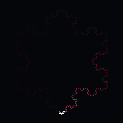
Koch Snowflake

FRACTALS / REWRITING / EDGE SUBSTITUTION

Helge von Koch, 1904

each side → four sides, each ⅓ the length
perimeter: L → (4/3)ⁿ·L
dimension: log 4 / log 3 ≈ 1.2619

Von Koch built it to show a curve with no tangent anywhere could come from elementary geometry, not only from the analytic monsters of Weierstrass. Every rewriting multiplies the perimeter by 4/3 while the area converges to 8/5 of the starting triangle — an infinitely long fence around a finite lawn, and the standard first example of a fractal.

Origin — H. von Koch, "Sur une courbe continue sans tangente, obtenue par une construction géométrique élémentaire", Arkiv för Matematik 1, 1904
Standing — Public domain — early 20th-century mathematics
Constants — Depth n draws 3·4ⁿ segments; past 5 the detail is finer than the plate
PL. 43

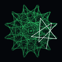
Maurer Rose

CURVES / POLAR / CHORD WALK

Peter M. Maurer, 1987

rose: r = sin(n·θ)
walk: θₖ = k·d°,  k = 0 … 360
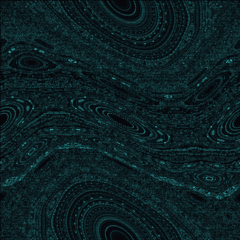
join consecutive walk points with chords

Take a rose curve, but instead of drawing it, walk around it in strides of d degrees and join the stops with straight chords. Maurer published it as a classroom exercise in line art; the figure changes completely with d, because the walk is really modular arithmetic on the circle. Prime-ish strides weave dense lace, while divisors of 360 collapse the whole thing to a polygon.

Origin — P. M. Maurer, "A Rose is a Rose…", The American Mathematical Monthly 94(7), 1987
Standing — Public domain — a construction on an 18th-century curve
Constants — 361 steps always return to the start, so the walk is a closed loop
HOUDINI · VEX — paste into a Detail Wrangle
// FORMA — PL. 43 · MAURER ROSE — Peter M. Maurer, 1987
//   rose: r = sin(n·θ)
//   walk: θₖ = k·d°,  k = 0 … 360
//   join consecutive walk points with chords
// Paste into a Detail Wrangle (Run Over: Detail), no inputs needed.
// Written from the published mathematics, not adapted from any code.
// Defaults are the published values; comments give the measured live range.
// https://forma-gen.com/#plate=maurer

float p_n = 6;         // 2 .. 8  · n — rose harmonic
float p_d = 71;        // 1 .. 179  · d — stride (deg)

// The plate's own colour: FORMA's CURVES accent as a cosine ramp,
// brightest near t = 0 and t = 1, near-black around t = 0.5.
vector forma_ramp(float t){
  return set(
    0.11 + 0.1196 * cos(6.28318530718 * (t + 0)),
    0.46 + 0.5 * cos(6.28318530718 * (t + 0.05)),
    0.2453 + 0.2667 * cos(6.28318530718 * (t + 0.1)));
}

// Two layers, as the plate draws them: the rose itself faint underneath, so
// the walk reads as chords of something — then the Maurer walk, 360 strides
// of d° joined point to point. Alpha carries the plate's own layering.
int forma_rose = 720;

float TAU = 6.28318530718;
int   n = int(rint(p_n));
// the rose, faint
int under = addprim(0, "polyline");
for (int i = 0; i <= forma_rose; i++){
    float th = float(i) / float(forma_rose) * TAU;
    float r  = sin(float(n) * th);
    // canvas y runs down; negated so the petals sit as the plate shows them
    int pt = addpoint(0, set(r * cos(th), -r * sin(th), 0.0));
    setpointattrib(0, "Cd", pt, forma_ramp(0.95));
    setpointattrib(0, "Alpha", pt, 0.14);
    addvertex(0, under, pt);
}
// the walk: closed after 360 strides, since 360·d° is a whole number of turns
int walk = addprim(0, "polyline");
for (int k = 0; k <= 360; k++){
    float th = float(k) * p_d * TAU / 360.0;
    float r  = sin(float(n) * th);
    int pt = addpoint(0, set(r * cos(th), -r * sin(th), 0.0));
    // colour runs along the walk inside the bright lobe of the ramp
    float u = float(k) / 360.0;
    setpointattrib(0, "Cd", pt, forma_ramp(0.8 + 0.3 * u));
    setpointattrib(0, "Alpha", pt, 1.0);
    addvertex(0, walk, pt);
}
PL. 44

Cardioid Chord Envelope

CURVES / ENVELOPE / MODULAR CHORDS

Luigi Cremona, 1862 · string-art tradition

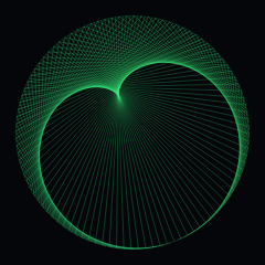
N points on a circle: Pₖ = e^(2πik/N)
chord: Pₖ → P₍m·k mod N₎
envelope: an epicycloid with m − 1 cusps

Join every point k on a circle to point m·k, working modulo N, and a curve nobody drew appears where the chords crowd together: the cardioid at m = 2, the nephroid at 3, an epicycloid of m − 1 cusps in general. Cremona described the construction; string artists have been hammering nails around circles and threading it ever since. The same picture hides in the Mandelbrot set, whose main cardioid is the m = 2 case.

Origin — L. Cremona, "Introduzione ad una teoria geometrica delle curve piane", 1862; folk practice as string art
Standing — Public domain — 19th-century geometry
Constants — Integer m resolves the envelope sharply; the sweep drifts through them
HOUDINI · VEX — paste into a Detail Wrangle
// FORMA — PL. 44 · CARDIOID CHORD ENVELOPE — Luigi Cremona, 1862 · string-art tradition
//   N points on a circle: Pₖ = e^(2πik/N)
//   chord: Pₖ → P₍m·k mod N₎
//   envelope: an epicycloid with m − 1 cusps
// Paste into a Detail Wrangle (Run Over: Detail), no inputs needed.
// Written from the published mathematics, not adapted from any code.
// Defaults are the published values; comments give the measured live range.
// https://forma-gen.com/#plate=cremona

float p_m   = 2;         // 2 .. 8  · m — multiplier
float p_n   = 200;       // 80 .. 320  · N — points
float p_off = 0;         // 0 .. 80  · shift — k·m + s

// The plate's own colour: FORMA's CURVES accent as a cosine ramp,
// brightest near t = 0 and t = 1, near-black around t = 0.5.
vector forma_ramp(float t){
  return set(
    0.11 + 0.1196 * cos(6.28318530718 * (t + 0)),
    0.46 + 0.5 * cos(6.28318530718 * (t + 0.05)),
    0.2453 + 0.2667 * cos(6.28318530718 * (t + 0.1)));
}

// String art on N nails: chord k → m·k + s for every k. The envelope is
// never drawn — the eye finds it where neighbouring chords crowd. A
// non-integer m lets the family slide between the classic figures; the
// additive shift s is a second family from the same nails.
int forma_circ = 128;

float TAU = 6.28318530718;
int n = int(rint(p_n));
// the nail circle, faint, as the plate strokes it
int circ = addprim(0, "polyline");
for (int i = 0; i <= forma_circ; i++){
    float th = float(i) / float(forma_circ) * TAU;
    int pt = addpoint(0, set(cos(th), -sin(th), 0.0));
    setpointattrib(0, "Cd", pt, forma_ramp(0.95));
    setpointattrib(0, "Alpha", pt, 0.22);
    addvertex(0, circ, pt);
}
// the chords — one two-point polyline each, colour running along k inside
// the bright lobe of the ramp
for (int k = 1; k <= n; k++){
    float a0 = float(k) * TAU / float(n);
    float a1 = (float(k) * p_m + p_off) % float(n) * TAU / float(n);
    vector col = forma_ramp(0.84 + 0.2 * float(k) / float(n));
    int chord = addprim(0, "polyline");
    // canvas y runs down; negated so the cusps sit as the plate shows them
    int pa = addpoint(0, set(cos(a0), -sin(a0), 0.0));
    int pb = addpoint(0, set(cos(a1), -sin(a1), 0.0));
    setpointattrib(0, "Cd", pa, col);
    setpointattrib(0, "Cd", pb, col);
    setpointattrib(0, "Alpha", pa, 0.38);
    setpointattrib(0, "Alpha", pb, 0.38);
    addvertex(0, chord, pa);
    addvertex(0, chord, pb);
}
PL. 45

Euler Spiral

CURVES / PARAMETRIC / LINEAR CURVATURE

Leonhard Euler, 1744 · Alfred Cornu, 1874

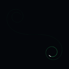
κ(s) = sᵏ⁻¹,  k = 2 is the Euler spiral
x(s) = ∫₀ˢ cos(uᵏ/k) du
y(s) = ∫₀ˢ sin(uᵏ/k) du

The curve whose curvature grows in exact proportion to the distance travelled along it — which is what a car traces when the driver turns the wheel at a constant rate. Euler found it studying a coiled spring; Cornu rediscovered it in the intensity integrals of diffraction. Railway and motorway engineers use the middle of it to ease straights into circular arcs, and each arm winds forever toward its Fresnel limit point without reaching it.

Origin — L. Euler, additamentum to "Methodus inveniendi lineas curvas", 1744; A. Cornu, on diffraction, 1874
Standing — Public domain — 18th-century analysis
Constants — Arc length sets how far each arm winds into its eye
HOUDINI · VEX — paste into a Detail Wrangle
// FORMA — PL. 45 · EULER SPIRAL — Leonhard Euler, 1744 · Alfred Cornu, 1874
//   κ(s) = sᵏ⁻¹,  k = 2 is the Euler spiral
//   x(s) = ∫₀ˢ cos(uᵏ/k) du
//   y(s) = ∫₀ˢ sin(uᵏ/k) du
// Paste into a Detail Wrangle (Run Over: Detail), no inputs needed.
// Written from the published mathematics, not adapted from any code.
// Defaults are the published values; comments give the measured live range.
// https://forma-gen.com/#plate=clothoid

float p_len  = 4.6;       // 2.5 .. 7  · arc length
float p_expo = 2;         // 1.2 .. 4  · k — curvature exponent

// The plate's own colour: FORMA's CURVES accent as a cosine ramp,
// brightest near t = 0 and t = 1, near-black around t = 0.5.
vector forma_ramp(float t){
  return set(
    0.11 + 0.1196 * cos(6.28318530718 * (t + 0)),
    0.46 + 0.5 * cos(6.28318530718 * (t + 0.05)),
    0.2453 + 0.2667 * cos(6.28318530718 * (t + 0.1)));
}

// The generalised Fresnel pair integrated with midpoint steps: curvature
// grows as s^(k−1), and k = 2 is the classic Euler spiral. The second arm is
// the first rotated half a turn — exact at k = 2, where the integrand pair
// is odd, and kept as the figure's symmetry elsewhere.
int forma_n = 1100;

float ds = p_len / float(forma_n);
float hx[], hy[];
float x = 0.0, y = 0.0;
for (int i = 0; i <= forma_n; i++){
    push(hx, x);  push(hy, y);
    float s = (float(i) + 0.5) * ds;
    x += cos(pow(s, p_expo) / p_expo) * ds;
    y += sin(pow(s, p_expo) / p_expo) * ds;
}
// second arm first, reversed, so the polyline runs end to end through zero
int prim = addprim(0, "polyline");
int total = 2 * forma_n + 1;
for (int i = 0; i < total; i++){
    int   j = i - forma_n;                       // −n … n
    float sgn = j < 0 ? -1.0 : 1.0;
    int   a = abs(j);
    // canvas y runs down; negated so the spiral winds as the plate shows it
    int pt = addpoint(0, set(sgn * hx[a], -sgn * hy[a], 0.0));
    // colour sweeps the bright lobe of the ramp along the curve
    float u = float(i) / float(total - 1);
    setpointattrib(0, "Cd", pt, forma_ramp(0.8 + 0.3 * u));
    addvertex(0, prim, pt);
}
PL. 46

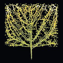
Pythagoras Tree

FRACTALS / RECURSION / SQUARE PAIR

Albert E. Bosman, 1942

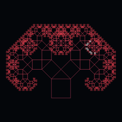
on each square, a right triangle of angle θ
two squares on its legs, scaled cos θ and sin θ
area per level: cos²θ + sin²θ = 1

Bosman, a Dutch engineering teacher, drew it by hand with compasses during the war and published it in a book about the wonder of plane geometry. Each square carries a right triangle on its shoulders and two smaller squares on the legs; the theorem itself guarantees every level adds exactly the same total area, while the silhouette turns from scaffolding into a wind-blown tree as the angle leaves 45°.

Origin — A. E. Bosman, drawn 1942; published in "Het wondere onderzoekingsveld der vlakke meetkunde", 1957
Standing — Public domain — a geometric construction
Constants — Depth doubles the square count per level; the angle sets the lean
PL. 47

L-System Plant

FRACTALS / L-SYSTEM / BRACKETED

Aristid Lindenmayer, 1968 · Przemysław Prusinkiewicz, 1990

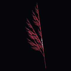
X → F−[[X]+X]+F[FX]−X
F → FF
δ = 22.5°

Lindenmayer was a biologist; the grammar was a model of how cells divide and differentiate, and the drawing came later. Rewrite the axiom a few times, then read the string as turtle instructions — F grows a shoot, brackets push and pop the turtle so a branch can return to its stem. This particular rule is the arching plant from The Algorithmic Beauty of Plants, and everything about its shape lives in the grammar, not the renderer.

Origin — A. Lindenmayer, "Mathematical models for cellular interactions in development", J. Theoretical Biology 18, 1968; the plant is figure 1.24f of Prusinkiewicz & Lindenmayer, "The Algorithmic Beauty of Plants", 1990
Standing — Public domain — a rewriting grammar from a scientific paper
Constants — Generations are locked: each one quadruples the string
PL. 48

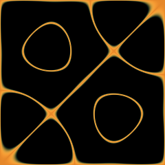
Chladni Figures

FIELDS / FIELD / STANDING WAVE

Ernst Chladni, 1787

u(x,y) = sin(mπx)·sin(nπy) + s·sin(nπx)·sin(mπy)
sand gathers where u = 0

Chladni bowed the edge of a sand-dusted brass plate and the grains leapt away from everything that moved, collecting along the still curves — the nodal lines of the standing wave. Napoleon put up a prize for the mathematics; Sophie Germain won it in 1816. The sine products here are the modes of the simply-supported rectangle, the drum-skin case that stands in for the brass, and s morphs between a mode pair sharing one frequency.

Origin — E. F. F. Chladni, "Entdeckungen über die Theorie des Klanges", Leipzig, 1787
Standing — Public domain — 18th-century acoustics
Constants — m and n pick the mode pair; the sweep drifts the mix between them
PL. 49

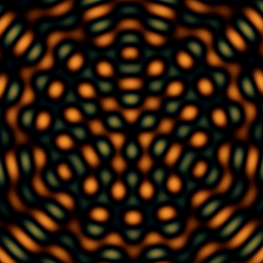
Wave Interference

FIELDS / FIELD / SUPERPOSITION

Thomas Young, 1801

ψ(p) = Σᵢ sin(2π·f·|p − sᵢ| − ωt)
nodes where the sum stays zero

Young argued light was a wave by showing two sources produce fringes — bands where the crests reinforce and lines where they always cancel. This plate rings several point sources at once: the instantaneous wave height maps antinodes bright in either phase, and the dark lanes between them are the nodes, the places that never move at all. Every hologram and every double-slit lecture demonstration is this picture.

Origin — T. Young, Bakerian Lecture, Philosophical Transactions of the Royal Society, 1802; the two-source demonstration followed in 1803
Standing — Public domain — the superposition principle
Constants — Sources sit on a ring; PHASE turns the ring per plate
PL. 50

Simplex Noise

FIELDS / NOISE / SIMPLEX LATTICE

Ken Perlin, 2001

skew to the simplex lattice: F = (√3−1)/2
n(p) = 70·Σᵢ (½ − |dᵢ|²)⁴ · (gᵢ · dᵢ)

Perlin rebuilt his own noise on a triangular lattice: three corners contribute instead of four, each through a radial kernel, so the cost grows linearly with dimension instead of exponentially. Then he patented it, and for two decades procedural graphics tiptoed around the construction — OpenSimplex exists specifically to avoid this formula. The patent lapsed in January 2022, and the original is finally free to write down.

Origin — K. Perlin, "Noise Hardware", SIGGRAPH course notes, 2001; the construction is laid out in detail by S. Gustavson, 2005
Patent — US6867776 — expired 8 January 2022
Standing — Free to use. Written from the published mathematics, not from any implementation.
PL. 51

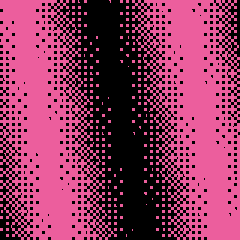
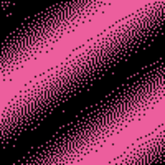
Ordered Dithering

COLOUR / DITHER / ORDERED MATRIX

Bryce Bayer, 1973

M₂ = [0 2; 3 1] / 4
M₂ₙ = [4M 4M+2; 4M+3 4M+1] / (2n)²
pixel lit where tone > M(x, y)

Bayer proved which threshold matrix spreads the on-dots as evenly as possible at every grey level, and his matrix has been the default ever since — newspaper halftones, 1-bit Macs, e-ink and the GPU path of this very plate. Each pixel consults only its own position, which is why the pattern is instant, parallel and perfectly stable while the tones slide beneath it.

Origin — B. E. Bayer, "An Optimum Method for Two-Level Rendition of Continuous-Tone Pictures", IEEE ICC, 1973
Standing — Public domain — a threshold matrix and an optimality proof
Constants — Order k gives the 2ᵏ×2ᵏ matrix; cells set the dot size
PL. 52

Error-Diffusion Dithering

COLOUR / DITHER / ERROR DIFFUSION

Robert W. Floyd & Louis Steinberg, 1976

quantise each pixel; pass the error on
ε → 7⁄16 →,  3⁄16 ↙,  5⁄16 ↓,  1⁄16 ↘

Where Bayer consults a fixed matrix, Floyd and Steinberg carry the rounding error to pixels not yet visited, so the mistakes cancel instead of accumulating. The result keeps detail ordered dithering loses — and it is inherently sequential: each pixel depends on every pixel before it, which is why this plate has no shader tab. The pair of dither plates is the whole parallel-versus-serial trade, drawn.

Origin — R. W. Floyd & L. Steinberg, "An Adaptive Algorithm for Spatial Greyscale", Proceedings of the Society for Information Display 17(2), 1976
Standing — Public domain — a quantisation algorithm from a published paper
Constants — The grid is locked: it sets both the dot size and the cost
PL. 53

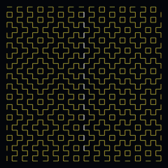
Hitomezashi Stitching

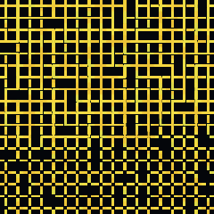
LATTICES / STITCHING / PARITY RULE

Traditional Japanese sashiko · Edo period onward

rows: stitch where (i + aⱼ) is even
columns: stitch where (j + bᵢ) is even
a, b ∈ {0,1} — two random sequences

Hitomezashi — "one-stitch" sashiko — sews single running stitches along the lines of a grid, and the entire cloth is determined by one bit per row and one bit per column: does that line start on or off. From those two coin-flip sequences, staircases, loops and long wandering paths emerge — structures the sewers of Edo-period Japan knew by eye long before percolation theory had names for them. Regenerate re-rolls the sequences.

Origin — Japanese needlework tradition; the parity description is the folk rule written down
Standing — Public domain — a craft pattern centuries old
Constants — Bias skews the two coin flips; at 0 or 1 the cloth collapses to stripes
PL. 54

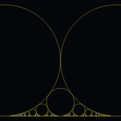
Ford Circles

LATTICES / NUMBER THEORY / TANGENT CIRCLES

Lester R. Ford, 1938 · after John Farey, 1816

for p/q in lowest terms:
centre (p/q, 1/2q²),  radius 1/2q²
tangent ⇔ |p·q′ − p′·q| = 1

Above every rational number sits a circle, tangent to the number line, its size falling with the square of the denominator. Ford noticed the miracle: no two circles ever overlap, and two touch exactly when their fractions are Farey neighbours — the whole arithmetic of mediants drawn as geometry. Between any two touching circles there is always a third, smaller one, forever, which is the number line telling you it is dense.

Origin — L. R. Ford, "Fractions", The American Mathematical Monthly 45(9), 1938; the fraction sequences are J. Farey, Philosophical Magazine, 1816
Standing — Public domain — number theory
Constants — Depth Q admits every reduced fraction with denominator up to Q
PL. 55

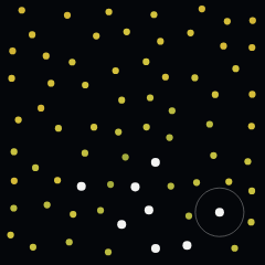
Poisson-Disk Sampling

LATTICES / SAMPLING / BLUE NOISE

Robert Bridson, 2007 · dart throwing after Robert L. Cook, 1986

no two samples closer than r
candidates ring an active sample: r ≤ d < 2r
k failures retire the sample

Random but never crowded: every sample keeps its neighbours at least r away, which is the "blue noise" the eye reads as even texture with no pattern. The photoreceptors of the monkey retina are packed this way, and renderers sample this way to trade aliasing for quiet noise. Cook proved why it works; Bridson found the linear-time construction this plate runs — grow outward from one seed, ringing each sample with candidates until it retires.

Origin — R. Bridson, "Fast Poisson Disk Sampling in Arbitrary Dimensions", SIGGRAPH sketches, 2007; R. L. Cook, "Stochastic Sampling in Computer Graphics", ACM Transactions on Graphics 5(1), 1986
Standing — Public domain — published algorithms, implemented from the papers
Constants — The gap is the whole definition; tries below ~10 leave visible holes
PL. 56

Cyclic Cellular Automaton

AUTOMATA / AUTOMATON / CYCLIC STATES

David Griffeath, 1988 · popularised by A. K. Dewdney, 1989

k states in a ring
s → s+1 (mod k) when ≥ θ von Neumann
neighbours already hold s+1

Rock-paper-scissors on a grid: every state is eaten by its successor, and the ring closes so nobody wins. From random debris the grid organises itself — droplets first, then spirals, which are the only structures that can feed forever — until every cell is turning in perfect lockstep. The plate detects that endgame and reseeds. The state ring maps straight onto the colour ramp, which is also a ring, so the wrap is seamless by construction.

Origin — D. Griffeath, University of Wisconsin, late 1980s; A. K. Dewdney, "Computer Recreations", Scientific American, August 1989
Standing — Public domain — a transition rule
Constants — Around 14 states the spirals win; far fewer and the debris never organises
PL. 57

Abelian Sandpile

AUTOMATA / AUTOMATON / SELF-ORGANISED

Per Bak, Chao Tang & Kurt Wiesenfeld, 1987

z ≥ 4 → z −= 4, one grain to each neighbour
grains leave at the boundary
topple order does not matter — the pile is abelian

Drop sand on one spot forever. Mostly nothing happens; sometimes a single grain sets off an avalanche that reorganises half the pile — and the avalanche sizes follow a power law with no preferred scale, which Bak, Tang and Wiesenfeld proposed as the origin of 1/f noise everywhere. The concentric fractal the centre-fed pile settles into looks designed; it is pure arithmetic. Abelian means the topple order is provably irrelevant, so the plate may defer work across frames without changing the result by one grain.

Origin — P. Bak, C. Tang & K. Wiesenfeld, "Self-Organized Criticality: An Explanation of 1/f Noise", Physical Review Letters 59, 1987
Standing — Public domain — a toppling rule
Constants — The pile reseeds the moment a grain first falls off the edge
PL. 58

Ising Model

AUTOMATA / STATISTICAL / SPIN LATTICE

Wilhelm Lenz, 1920 · Ernst Ising, 1925 · Metropolis et al., 1953

E = −Σ⟨ij⟩ sᵢ·sⱼ − B·Σ sᵢ,  s = ±1
flip with probability min(1, e^(−ΔE/T))
T_c = 2 / ln(1 + √2) ≈ 2.269 at B = 0

Ising solved the one-dimensional chain for his 1925 thesis, found no phase transition, and concluded the model explained nothing; Onsager proved in 1944 that two dimensions transition sharply at T_c. This plate rides the temperature slowly through that point, both directions, forever: above it the spins are noise, below it domains freeze out and coarsen, and the crossing is announced each way. The sampling is Metropolis 1953 — the algorithm that named Monte Carlo methods.

Origin — E. Ising, Zeitschrift für Physik 31, 1925; N. Metropolis, A. & M. Rosenbluth, A. & E. Teller, J. Chemical Physics 21, 1953; T_c from L. Onsager, Physical Review 65, 1944
Standing — Public domain — statistical mechanics
Constants — Span sets how far the temperature rides either side of critical
PL. 59

Brian’s Brain

AUTOMATA / AUTOMATON / 3-STATE

Brian Silverman, 1984

off → firing with exactly 2 firing neighbours
firing → refractory → off
(Moore neighbourhood)

Conway’s rules with a refractory period: a cell that fires must rest one generation before it can fire again, the way a neuron must. That one change abolishes still lifes — nothing in this universe can stand still — so the whole grid runs with gliders, wavefronts and colliding storms indefinitely. Silverman built it while writing educational software; Toffoli and Margolus made it a standard exhibit of what one extra state buys.

Origin — Devised by Brian Silverman, 1984; described in Toffoli & Margolus, "Cellular Automata Machines", MIT Press, 1987
Standing — Public domain — a transition rule
Constants — The storm is deterministic per seed; it reseeds on burnout or after its run
PL. 60

Double Pendulum

CURVES / MECHANICS / CHAOTIC

Classical Lagrangian mechanics · after Euler and Lagrange

two rods, two bobs, one pivot
θ̈₁, θ̈₂ from the Euler–Lagrange equations
no closed form — the motion must be integrated

One pendulum is the clock; two, hinged together, are chaos you can build with a hacksaw. The equations fall straight out of the Lagrangian and cannot be solved — only integrated — and two starts a hair apart diverge until they share nothing but energy. This is the demonstration piece of sensitive dependence: the trail the lower bob leaves is a chaotic attractor being drawn by actual mechanics, live.

Origin — The compound pendulum goes back to the Bernoullis and Euler; the Lagrangian formulation is J.-L. Lagrange, "Mécanique analytique", 1788
Standing — Public domain — classical mechanics
Constants — PHASE varies the launch angle, so no two plates swing alike
HOUDINI · VEX — paste into a Detail Wrangle
// FORMA — PL. 60 · DOUBLE PENDULUM — Classical Lagrangian mechanics · after Euler and Lagrange
//   two rods, two bobs, one pivot
//   θ̈₁, θ̈₂ from the Euler–Lagrange equations
//   no closed form — the motion must be integrated
// Paste into a Detail Wrangle (Run Over: Detail), no inputs needed.
// Written from the published mathematics, not adapted from any code.
// Defaults are the published values; comments give the measured live range.
// https://forma-gen.com/#plate=pendulum

float p_mass   = 1;         // 0.3 .. 2  · m₂ / m₁
float p_len    = 1;         // 0.5 .. 1.5  · l₂ / l₁
float p_launch = 0.55;      // 0.2 .. 0.95  · launch angle (× π)

// The plate's own colour: FORMA's CURVES accent as a cosine ramp,
// brightest near t = 0 and t = 1, near-black around t = 0.5.
vector forma_ramp(float t){
  return set(
    0.11 + 0.1196 * cos(6.28318530718 * (t + 0)),
    0.46 + 0.5 * cos(6.28318530718 * (t + 0.05)),
    0.2453 + 0.2667 * cos(6.28318530718 * (t + 0.1)));
}

// The Euler–Lagrange equations for two rods under RK4, m₁ = l₁ = 1, and the
// second bob's trail emitted as the path. In a chaotic system the launch
// angle is the parameter: low energy gives a lazy lissajous trail, high
// enough gives full flips.
int   forma_steps = 6000;    // dt = 0.01, recording every second step
float forma_dt    = 0.01;
float forma_g     = 9.81;

vector4 forma_deriv(vector4 st; float m2, l2, g){
    float a1 = st.x, a2 = st.y, w1 = st.z, w2 = st.w;
    float d = a1 - a2;
    float den = 2.0 + m2 - m2 * cos(2.0 * d);
    float dw1 = (-g * (2.0 + m2) * sin(a1) - m2 * g * sin(a1 - 2.0 * a2)
                 - 2.0 * sin(d) * m2 * (w2 * w2 * l2 + w1 * w1 * cos(d))) / den;
    float dw2 = (2.0 * sin(d) * (w1 * w1 * (1.0 + m2) + g * (1.0 + m2) * cos(a1)
                 + w2 * w2 * l2 * m2 * cos(d))) / (l2 * den);
    return set(w1, w2, dw1, dw2);
}

vector4 st = set(3.14159265359 * p_launch, 3.14159265359 * 0.95, 0.0, 0.0);
int prim = addprim(0, "polyline");
for (int i = 0; i < forma_steps; i++){
    vector4 k1 = forma_deriv(st, p_mass, p_len, forma_g);
    vector4 k2 = forma_deriv(st + k1 * forma_dt / 2.0, p_mass, p_len, forma_g);
    vector4 k3 = forma_deriv(st + k2 * forma_dt / 2.0, p_mass, p_len, forma_g);
    vector4 k4 = forma_deriv(st + k3 * forma_dt, p_mass, p_len, forma_g);
    st += (k1 + 2.0 * k2 + 2.0 * k3 + k4) * forma_dt / 6.0;
    if (!isfinite(st.x) || !isfinite(st.y)) break;
    if (i % 2 == 0) continue;
    // the tip in world terms: rods hang downward, Houdini y-up
    float tx = sin(st.x) + p_len * sin(st.y);
    float ty = -(cos(st.x) + p_len * cos(st.y));
    int pt = addpoint(0, set(tx, ty, 0.0));
    // colour sweeps the bright lobe of the ramp along the trail
    float u = float(i) / float(forma_steps);
    setpointattrib(0, "Cd", pt, forma_ramp(0.8 + 0.3 * u));
    addvertex(0, prim, pt);
}
PL. 61

Three-Body Figure-Eight

CURVES / MECHANICS / CHOREOGRAPHY

Cristopher Moore, 1993 · Chenciner & Montgomery, 2000

ẍᵢ = Σⱼ (xⱼ − xᵢ)/|xⱼ − xᵢ|³
three equal masses, one shared orbit
x₁(t) = x₂(t + T/3) = x₃(t + 2T/3)

Three equal masses chasing each other around a single figure-eight, each a third of a period behind the next — a choreography, in the technical term the discovery created. Moore found it numerically; Chenciner and Montgomery proved it exists with variational calculus, to considerable astonishment, since almost every three-body arrangement tears itself apart. It has no dials: perturb the initial conditions and the braid dissolves, so the sliders here drive the clock and the comet, not the orbit.

Origin — C. Moore, "Braids in Classical Dynamics", Physical Review Letters 70, 1993; A. Chenciner & R. Montgomery, Annals of Mathematics 152, 2000; initial conditions as refined numerically by Carles Simó
Standing — Public domain — celestial mechanics
Constants — One period is integrated once and traced forever
HOUDINI · VEX — paste into a Detail Wrangle
// FORMA — PL. 61 · THREE-BODY FIGURE-EIGHT — Cristopher Moore, 1993 · Chenciner & Montgomery, 2000
//   ẍᵢ = Σⱼ (xⱼ − xᵢ)/|xⱼ − xᵢ|³
//   three equal masses, one shared orbit
//   x₁(t) = x₂(t + T/3) = x₃(t + 2T/3)
// Paste into a Detail Wrangle (Run Over: Detail), no inputs needed.
// Written from the published mathematics, not adapted from any code.
// Defaults are the published values; comments give the measured live range.
// https://forma-gen.com/#plate=threebody

float p_speed = 0.8;       // 0.2 .. 2  · orbit rate
float p_tail  = 0.5;       // 0.1 .. 0.9  · comet length

// The plate's own colour: FORMA's CURVES accent as a cosine ramp,
// brightest near t = 0 and t = 1, near-black around t = 0.5.
vector forma_ramp(float t){
  return set(
    0.11 + 0.1196 * cos(6.28318530718 * (t + 0)),
    0.46 + 0.5 * cos(6.28318530718 * (t + 0.05)),
    0.2453 + 0.2667 * cos(6.28318530718 * (t + 0.1)));
}

// Simó's initial conditions for the figure-eight, one full period under RK4.
// The curve is shared: bodies 2 and 3 ride the same points a third of a lap
// apart, so one closed polyline is the whole choreography.
// waived: speed, tail — they pace the plate's comet, and geometry has no clock
int   forma_n = 3000;
float forma_T = 6.32591398;

function float[] forma_accel(float s0[]){
    float d[];
    resize(d, 12);
    for (int i = 0; i < 3; i++){ d[i * 2] = s0[6 + i * 2]; d[i * 2 + 1] = s0[7 + i * 2]; }
    for (int i = 0; i < 3; i++){
        float ax = 0.0, ay = 0.0;
        for (int j = 0; j < 3; j++){
            if (i == j) continue;
            float dx = s0[j * 2] - s0[i * 2], dy = s0[j * 2 + 1] - s0[i * 2 + 1];
            float r = sqrt(dx * dx + dy * dy);
            ax += dx / (r * r * r);  ay += dy / (r * r * r);
        }
        d[6 + i * 2] = ax;  d[7 + i * 2] = ay;
    }
    return d;
}
function float[] forma_step(float a[]; float b[]; float sc){
    float o[];
    resize(o, 12);
    for (int i = 0; i < 12; i++) o[i] = a[i] + b[i] * sc;
    return o;
}

float st[] = { 0.97000436, -0.24308753, -0.97000436, 0.24308753, 0.0, 0.0,
               0.46620368, 0.43236573, 0.46620368, 0.43236573,
               -0.93240737, -0.86473146 };
float dt = forma_T / float(forma_n);
int prim = addprim(0, "polyline");
for (int i = 0; i < forma_n; i++){
    float k1[] = forma_accel(st);
    float k2[] = forma_accel(forma_step(st, k1, dt / 2.0));
    float k3[] = forma_accel(forma_step(st, k2, dt / 2.0));
    float k4[] = forma_accel(forma_step(st, k3, dt));
    for (int j = 0; j < 12; j++)
        st[j] += (k1[j] + 2.0 * k2[j] + 2.0 * k3[j] + k4[j]) * dt / 6.0;
    // canvas y runs down; negated so the eight lies as the plate shows it
    int pt = addpoint(0, set(st[0], -st[1], 0.0));
    // colour sweeps the bright lobe of the ramp around the lap
    float u = float(i) / float(forma_n);
    setpointattrib(0, "Cd", pt, forma_ramp(0.8 + 0.3 * u));
    addvertex(0, prim, pt);
}
PL. 62

Space Colonisation

LATTICES / GROWTH / SPACE COLONISATION

Adam Runions, Brendan Lane & Przemysław Prusinkiewicz, 2007

each attractor pulls its nearest node
nodes step toward the mean pull
attractors die inside the kill radius

Scatter points where a plant could grow, then let the branches compete for them: every attractor tugs on its nearest node, each node steps toward the average tug, and any attractor approached closely enough is consumed. That is the whole algorithm, and it produces leaf venation, tree crowns and root systems depending only on how the attractors are scattered. Growth claims territory — hence colonisation — and when the field is spent, the plate scatters a fresh one.

Origin — A. Runions, B. Lane & P. Prusinkiewicz, "Modeling Trees with a Space Colonization Algorithm", Eurographics Workshop on Natural Phenomena, 2007
Standing — Public domain — implemented from the published description
Constants — The attractor count is locked: it is the cost of every growth step
PL. 63

Metaballs

FIELDS / ISO-SURFACE / SUMMED FALLOFF

James Blinn, 1982

D(r) = b·e^(−a·r²)
F(p) = Σᵢ D(|p − cᵢ|)
draw the curves where F = threshold

Blinn was rendering electron density maps for molecular models and needed surfaces that merged where atoms overlapped. Each centre contributes a Gaussian falloff, the field is simply their sum, and the surface is wherever that sum crosses a threshold — so two approaching blobs bulge toward one another and fuse without any special case for the join. He called them blobby models; everyone else calls them metaballs.

Origin — J. F. Blinn, "A Generalization of Algebraic Surface Drawing", ACM Transactions on Graphics 1(3), 1982
Standing — Public domain — a summation of exponentials
Contours — Extracted with marching squares (Lorensen & Cline, 1987, in its 2D form), which is why this field exports as real vector
PL. 64

Curl Noise

FIELDS / FIELD / DIVERGENCE-FREE

Robert Bridson, Jim Houriham & Marcus Nordenstam, 2007

v = ∇ × ψ,  in 2D: v = (∂ψ/∂y, −∂ψ/∂x)
∇ · v = 0 identically

Take a noise field, call it a stream function, and use its perpendicular gradient as a velocity. The curl of any field is divergence-free by construction, so this flow can never compress: particles swirl indefinitely and never pile into the sinks that an angle read straight out of noise always produces. Bridson introduced it for smoke and water that had to look turbulent without being simulated. Compare plate 23, which does read the angle directly — the difference is visible as bunching.

Origin — R. Bridson, J. Houriham & M. Nordenstam, "Curl-Noise for Procedural Fluid Flow", ACM Transactions on Graphics 26(3), SIGGRAPH 2007
Standing — Public domain — a vector identity applied to noise
Constants — Particle count is locked: it is the cost of every advection step
PL. 65

Lyapunov Fractal

FRACTALS / EXPONENT / FORCED LOGISTIC

Mario Markus & Benno Hess, 1989

xₙ₊₁ = rₙ·xₙ(1 − xₙ),  rₙ ∈ {a, b} by a repeating word
λ = lim (1/N)·Σ ln|rₙ(1 − 2xₙ)|
λ < 0 stable · λ > 0 chaotic

Drive the logistic map with two growth rates instead of one, alternating between them on a fixed repeating word, and plot the Lyapunov exponent over the (a, b) plane. Negative means nearby starts converge and the population settles; positive means they separate and it never does. Markus and Hess found the boundary between those regions is not a curve but an intricate structure of interlocking arms, and the shape depends entirely on the word — swapping AB for AABB rebuilds the picture.

Origin — M. Markus & B. Hess, "Lyapunov Exponents of the Logistic Map with Periodic Forcing", Computers & Graphics 13(4), 1989
Standing — Public domain — an exponent of a published map
Cost — Per-pixel iteration, in mandelbrot’s class. Iteration count is locked, and the shader is why this renders sharp.
PL. 66

Buddhabrot

FRACTALS / ESCAPE ORBIT / DENSITY

Melinda Green, 1993

for c that escape: plot every zₙ of the orbit
z₀ = 0,  zₙ₊₁ = zₙ² + c
density of visits, not escape time

The Mandelbrot set rendered inside out. Instead of colouring each c by how fast it escapes, sample points at random, throw away the ones that stay bounded, and plot the whole trajectory of the ones that get away. Where those escaping orbits linger, the plate brightens. Green found the resulting figure — a seated form with a halo — while experimenting on a mailing list in 1993, and it looks nothing like the set it comes from.

Origin — Melinda Green, 1993, circulated on the sci.fractals newsgroup
Standing — Public domain — a rendering method for a public-domain set
Constants — Orbit length bounds are locked: they set both the figure and the cost
PL. 67

Penrose Tiling

LATTICES / TILING / APERIODIC

Roger Penrose, 1974 · after Robinson and de Bruijn

deflate each Robinson triangle by φ = (1+√5)/2
acute → one acute + one obtuse
obtuse → two obtuse + one acute

Two rhombs that tile the plane and can never tile it periodically. Penrose found the set in 1974; the proof that no arrangement of them ever repeats is what made it famous, and Shechtman’s quasicrystals turned it from recreation into physics a decade later. This plate builds it by deflation — start with ten Robinson triangles around a point and subdivide each in the golden ratio, forever. Every vertex configuration you see is forced.

Origin — R. Penrose, "The Rôle of Aesthetics in Pure and Applied Mathematical Research", Bull. Inst. Math. Appl. 10, 1974; de Bruijn gave the pentagrid construction in 1981
Patent — US4133152, granted 1979 to Penrose, covering the tiles as a puzzle — long expired
Standing — Free to use. Built here by triangle deflation, from the published rule.
PL. 68

Wave Function Collapse

LATTICES / CONSTRAINT / MIN ENTROPY

Maxim Gumin, 2016 · analysed by Karth & Smith, 2017

every cell holds the set of tiles still possible
observe: collapse the lowest-entropy cell
propagate: strike neighbours that no longer fit

A constraint solver that behaves like a texture generator. Every cell starts holding every tile; repeatedly commit the cell with the fewest options left to one of them at random, then strike from its neighbours whatever no longer fits, until the grid is decided. Karth and Smith identified it as ordinary constraint propagation under a minimum-entropy heuristic — which is what makes its notorious failure possible, since nothing backtracks. Not on this tile set, though. Measured over 170 waves it never once contradicted: when tiles agree by matching a socket across a shared edge, propagating to arc-consistency is already enough to guarantee a solution exists. The contradictions WFC is known for need constraints that reach further than one edge.

Origin — Maxim Gumin, 2016. The algorithm is implemented here from the description in I. Karth & A. M. Smith, "WaveFunctionCollapse is Constraint Solving in the Wild", Foundations of Digital Games, 2017 — not from the reference implementation.
Standing — Public domain — a constraint-propagation procedure
Tiles — The simple tiled model. The eleven-tile connector set and its edge-socket adjacency are this atlas’s own, not anyone’s asset pack.
PL. 69

Weierstrass Function

CURVES / SERIES / PATHOLOGICAL

Karl Weierstrass, 1872 · G. H. Hardy, 1916

W(x) = Σ aⁿ cos(bⁿ π x)
0 < a < 1, b odd integer, ab > 1 + 3π/2  (Weierstrass, 1872)
0 < a < 1, b real, ab ≥ 1  (Hardy, 1916)
continuous everywhere · differentiable nowhere

The function that ended the belief that a continuous curve must have a tangent somewhere — Weierstrass read it to the Berlin Academy and the century’s geometers called it a scandal. Every term is a smooth cosine; the sum has a corner at every point. Weierstrass needed b to be an odd integer and ab past 1 + 3π/2; Hardy pulled both away, leaving ab ≥ 1 for real b, and that is the condition on the plate. What the canvas shows is necessarily a partial sum, because any finite sum is smooth and the pathology lives only in the limit — terms whose frequency passes the pixel grid are dropped, since past that they alias into noise the mathematics never contained.

Origin — K. Weierstrass, read to the Königlich Preussische Akademie der Wissenschaften, Berlin, 18 July 1872 — recorded in the Monatsberichte for 1872, p. 560; G. H. Hardy, "Weierstrass’s non-differentiable function", Trans. AMS 17 (1916), 301–325, dropped the odd-integer requirement on b and weakened ab > 1 + 3π/2 to ab ≥ 1
Standing — Public domain — 19th-century analysis
Constants — The term count is set by resolution, not by a dial: a finite sum is smooth, so more terms than the pixels resolve would claim a depth the plate cannot show. Both sliders stay inside Hardy’s condition across their whole range — the weakest corner, a = 0.34 against b = 3, still gives ab = 1.02
HOUDINI · VEX — paste into a Detail Wrangle
// FORMA — PL. 69 · WEIERSTRASS FUNCTION — Karl Weierstrass, 1872 · G. H. Hardy, 1916
//   W(x) = Σ aⁿ cos(bⁿ π x)
//   0 < a < 1, b odd integer, ab > 1 + 3π/2  (Weierstrass, 1872)
//   0 < a < 1, b real, ab ≥ 1  (Hardy, 1916)
//   continuous everywhere · differentiable nowhere
// Paste into a Detail Wrangle (Run Over: Detail), no inputs needed.
// Written from the published mathematics, not adapted from any code.
// Defaults are the published values; comments give the measured live range.
// https://forma-gen.com/#plate=weierstrass

float p_a = 0.55;      // 0.34 .. 0.68  · a — amplitude ratio
float p_b = 5;         // 3 .. 9  · b — frequency ratio

// The plate's own colour: FORMA's CURVES accent as a cosine ramp,
// brightest near t = 0 and t = 1, near-black around t = 0.5.
vector forma_ramp(float t){
  return set(
    0.11 + 0.1196 * cos(6.28318530718 * (t + 0)),
    0.46 + 0.5 * cos(6.28318530718 * (t + 0.05)),
    0.2453 + 0.2667 * cos(6.28318530718 * (t + 0.1)));
}

// Continuous everywhere, differentiable nowhere. Depth is bounded by what
// the samples can hold: bⁿ stays under a quarter of the sample count so the
// top term still renders as oscillation rather than aliasing into noise the
// mathematics never contained — the plate's own ceiling.
int forma_n = 1600;

int terms = max(2, int(floor(1.0 + log(float(forma_n) / 4.0) / log(p_b))));
// Σ|aⁿ| — normalising by it keeps every (a, b) on the same amplitude
float norm = (1.0 - pow(p_a, terms)) / (1.0 - p_a);
int prim = addprim(0, "polyline");
for (int i = 0; i <= forma_n; i++){
    float x = float(i) / float(forma_n) * 2.0 - 1.0;
    float y = 0.0;
    for (int k = 0; k < terms; k++)
        y += pow(p_a, k) * cos(pow(p_b, k) * 3.14159265359 * x);
    // the graph is drawn y-up already; no flip needed
    int pt = addpoint(0, set(x, y / norm, 0.0));
    // colour sweeps the bright lobe of the ramp along the graph
    float u = float(i) / float(forma_n);
    setpointattrib(0, "Cd", pt, forma_ramp(0.8 + 0.3 * u));
    addvertex(0, prim, pt);
}
PL. 70

Takagi Curve

CURVES / SERIES / MIDPOINT TENT

Teiji Takagi, 1901

T(x) = Σ wⁿ s(2ⁿ x)
s(x) = distance from x to the nearest integer
w = ½ is the blancmange

Takagi’s simpler route to Weierstrass’s scandal, published as "a simple example of the continuous function without derivative": stack tent maps, each twice the frequency and a fraction of the height of the last. At w = ½ the sum is the blancmange curve, named for the pudding; the weight slides the family from nearly-smooth toward a jagged ridge, and the plate builds it a term at a time because the construction is the exhibit.

Origin — T. Takagi, "A simple example of the continuous function without derivative", Tokyo Sugaku-Butsurigakkwai Hokoku (Proc. Phys.-Math. Soc. Japan) 1, F176–F177 — the volume is dated 1901 and the paper is just as often cited as 1903; the w ≠ ½ family is Takagi–Landsberg, after G. Landsberg, Jahresber. Deutsch. Math.-Verein. 17 (1908), 46–51
Standing — Public domain — early 20th-century analysis
Constants — Term count is resolution-bound, as on PL. 69: each term doubles in frequency, and past the pixel grid there is nothing left to draw
HOUDINI · VEX — paste into a Detail Wrangle
// FORMA — PL. 70 · TAKAGI CURVE — Teiji Takagi, 1901
//   T(x) = Σ wⁿ s(2ⁿ x)
//   s(x) = distance from x to the nearest integer
//   w = ½ is the blancmange
// Paste into a Detail Wrangle (Run Over: Detail), no inputs needed.
// Written from the published mathematics, not adapted from any code.
// Defaults are the published values; comments give the measured live range.
// https://forma-gen.com/#plate=takagi

float p_w = 0.5;       // 0.4 .. 0.8  · w — term weight

// The plate's own colour: FORMA's CURVES accent as a cosine ramp,
// brightest near t = 0 and t = 1, near-black around t = 0.5.
vector forma_ramp(float t){
  return set(
    0.11 + 0.1196 * cos(6.28318530718 * (t + 0)),
    0.46 + 0.5 * cos(6.28318530718 * (t + 0.05)),
    0.2453 + 0.2667 * cos(6.28318530718 * (t + 0.1)));
}

// The blancmange at full depth: ten tent-map terms, which is the sample
// floor — 2¹⁰ oscillations across 1400 samples is where the top term stops
// rendering as shape. The plate reveals the terms one by one; the geometry
// is the finished pathology.
int forma_n   = 1400;
int forma_top = 10;

// peak of Σ wⁿ·s(2ⁿx) is bounded by Σ wⁿ/2; normalising keeps every weight
// on the same baseline
float norm = (1.0 - pow(p_w, forma_top)) / (1.0 - p_w) * 0.5;
int prim = addprim(0, "polyline");
for (int i = 0; i <= forma_n; i++){
    float x = float(i) / float(forma_n);
    float y = 0.0;
    for (int k = 0; k < forma_top; k++){
        float sx = x * pow(2.0, k);      // VEX has no shift operator
        y += pow(p_w, k) * abs(sx - rint(sx));
    }
    // the graph is drawn y-up already; no flip needed
    int pt = addpoint(0, set(x, y / norm, 0.0));
    // colour sweeps the bright lobe of the ramp along the graph
    float u = float(i) / float(forma_n);
    setpointattrib(0, "Cd", pt, forma_ramp(0.8 + 0.3 * u));
    addvertex(0, prim, pt);
}
PL. 71

Gosper Flowsnake

FRACTALS / L-SYSTEM / HEX SUBSTITUTION

William Gosper, 1973 · via Martin Gardner

A → A−B−−B+A++AA+B−
B → +A−BB−−B−A++A+B
turn 60° · both symbols step forward

Gosper’s space-filling curve on the hexagonal lattice, which Gardner introduced to the world as the "flowsnake" — a spoonerism of snowflake — and the name stuck. Seven copies of the path tile a hexagonal island that is itself one cell of the next scale up, so the curve fills the plane the way hilbert’s fills the square — but with a boundary that is fractal rather than straight, the Gosper island, of dimension log 3 / log √7 ≈ 1.129. One rewrite per generation multiplies the path by seven.

Origin — R. W. Gosper, 1973; published to a wide audience in M. Gardner, "In which ‘monster’ curves force redefinition of the word ‘curve’", Mathematical Games, Scientific American 235(6), December 1976 — later reprinted as "Mandelbrot’s Fractals" in Penrose Tiles to Trapdoor Ciphers. Mandelbrot renamed the curve Peano–Gosper and the tile the Gosper island in Fractals, 1977
Standing — Public domain — a curve construction
Constants — Generations are locked from regenerate: each multiplies the path sevenfold, which is a cost dial, not a look dial
PL. 72

Lévy C Curve

FRACTALS / REWRITING / SYMMETRIC FOLD

Ernesto Cesàro, 1906 · Georg Faber, 1910 · Paul Lévy, 1938

F → +F−−F+   (turn θ, 45° is the C)
every segment folds outward each generation
dimension → 2 as the folds close

Fold every segment of a line into a right-angle tent, forever, and the C curve appears — Cesàro described it first and Faber analysed the same family, both for its differentiability; Lévy was the one who set out its self-similarity and the geometric construction, and the name went to him. It is the koch construction’s wilder sibling: koch’s bump keeps the curve simple, while the C’s symmetric fold makes it cross itself into a paved, furred braid. The angle walks the Cesàro–Faber family — de Rham curves, with the classical C at 45°.

Origin — E. Cesàro, "Fonctions continues sans dérivée", Archiv der Mathematik und Physik (3) 38 (1906), 57–63; G. Faber, 1910, on the same family; P. Lévy, "Les courbes planes ou gauches et les surfaces composées de parties semblables au tout", Journal de l’École Polytechnique, 1938, 227–247 and 249–291, which is where the self-similar construction and the name come from
Standing — Public domain — early 20th-century geometry
Constants — Generations are locked: each doubles the segment count. The fold angle is free — the whole range is alive
PL. 73

Gibbs Phenomenon

CURVES / SERIES / FOURIER PARTIAL SUM

Henry Wilbraham, 1848 · J. Willard Gibbs, 1899 · named by Maxime Bôcher, 1906

fₙ(x) = (4/π) Σₖ₌₁ⁿ sin((2k−1)x)/(2k−1)
peak → (2/π)·Si(π) ≈ 1.178980
overshoot → 0.0894899 of the jump
it never dies — it only narrows

Sum the odd harmonics of a square wave and the corners grow horns: about nine per cent of the jump, and adding terms makes them thinner but never shorter — the partial sums converge everywhere except in the one sense the eye measures. The name is the least accurate part of it. Wilbraham had published the whole effect fifty years earlier and been ignored; Gibbs came to it through the Nature argument over Michelson’s harmonic analyser, and his first note there missed the overshoot entirely — it was his 1899 correction that described it. The name was Bôcher’s, seven years later still. The credit line here runs in the order the work actually happened. The swept harmonic count is the exhibit: watch the wave sharpen and the horns refuse to leave.

Origin — H. Wilbraham, "On a certain periodic function", Cambridge & Dublin Math. Journal 3 (1848), 198–201, unnoticed for decades; the effect resurfaced in the 1898 Nature exchange between A. A. Michelson and A. E. H. Love over Michelson’s harmonic analyser. J. W. Gibbs, "Fourier’s Series", Nature 59 (1898), 200, did not yet identify the overshoot; his correction, Nature 59 (1899), 606, did. M. Bôcher, "Introduction to the theory of Fourier’s series", Annals of Mathematics (2) 7 (1906), 81–152, gave the first full treatment and coined "Gibbs phenomenon"
Standing — Public domain — 19th-century analysis
Constants — The square wave underneath is the target the sums chase; it stays faint so the horns read against it. The limit peak is (2/π)·Si(π), the Wilbraham–Gibbs constant
HOUDINI · VEX — paste into a Detail Wrangle
// FORMA — PL. 73 · GIBBS PHENOMENON — Henry Wilbraham, 1848 · J. Willard Gibbs, 1899 · named by Maxime Bôcher, 1906
//   fₙ(x) = (4/π) Σₖ₌₁ⁿ sin((2k−1)x)/(2k−1)
//   peak → (2/π)·Si(π) ≈ 1.178980
//   overshoot → 0.0894899 of the jump
//   it never dies — it only narrows
// Paste into a Detail Wrangle (Run Over: Detail), no inputs needed.
// Written from the published mathematics, not adapted from any code.
// Defaults are the published values; comments give the measured live range.
// https://forma-gen.com/#plate=gibbs

float p_terms  = 24;        // 1 .. 48  · n — odd harmonics
float p_cycles = 2;         // 1 .. 4  · cycles shown

// The plate's own colour: FORMA's CURVES accent as a cosine ramp,
// brightest near t = 0 and t = 1, near-black around t = 0.5.
vector forma_ramp(float t){
  return set(
    0.11 + 0.1196 * cos(6.28318530718 * (t + 0)),
    0.46 + 0.5 * cos(6.28318530718 * (t + 0.05)),
    0.2453 + 0.2667 * cos(6.28318530718 * (t + 0.1)));
}

// The square wave faint underneath — the structure the sums are chasing —
// and the partial sum over it, normalised so the square sits at ±1. The
// horns overshoot by design: ~8.9% of the jump, and adding terms only
// narrows them. It never dies. Alpha carries the plate's own layering.
int forma_n = 1200;

float TAU = 6.28318530718;
int terms = max(1, int(rint(p_terms)));
// the target square wave, faint
int under = addprim(0, "polyline");
for (int i = 0; i <= forma_n; i++){
    float x = p_cycles * TAU * float(i) / float(forma_n);
    float s = sin(x);
    float sq = s == 0.0 ? 1.0 : sign(s);
    int pt = addpoint(0, set(float(i) / float(forma_n), sq, 0.0));
    setpointattrib(0, "Cd", pt, forma_ramp(0.95));
    setpointattrib(0, "Alpha", pt, 0.16);
    addvertex(0, under, pt);
}
// the partial sum — the graph is drawn y-up already; no flip needed
int prim = addprim(0, "polyline");
for (int i = 0; i <= forma_n; i++){
    float x = p_cycles * TAU * float(i) / float(forma_n);
    float y = 0.0;
    for (int k = 1; k <= terms; k++)
        y += sin(float(2 * k - 1) * x) / float(2 * k - 1);
    int pt = addpoint(0, set(float(i) / float(forma_n), y * 4.0 / 3.14159265359, 0.0));
    setpointattrib(0, "Cd", pt, forma_ramp(0.94));
    setpointattrib(0, "Alpha", pt, 1.0);
    addvertex(0, prim, pt);
}
PL. 74

Recamán Sequence

CURVES / SEQUENCE / GREEDY WALK

Bernardo Recamán Santos, 1991 · via N. J. A. Sloane

a₀ = s
aₙ = aₙ₋₁ − n   if positive and unvisited
aₙ = aₙ₋₁ + n   otherwise

Step backwards if you can, forwards if you must, with strides that grow by one each time. Recamán sent the sequence to Sloane in 1991; it became OEIS A005132, and Sloane has called it a favourite. Whether every number is eventually visited is still open — the smallest one not known to appear is 852,655. The drawing is the familiar one, consecutive terms joined by semicircles alternating above and below the number line, and the reveal walks it stride by stride because the rule is the exhibit.

Origin — B. Recamán Santos, in a 1991 letter to N. J. A. Sloane; OEIS A005132
Standing — Public domain — an integer sequence and its folk rendering
Drawing — The alternating semicircles are not the OEIS’s own plot: that rendering was popularised by Numberphile’s "The Slightly Spooky Recamán Sequence", 14 January 2018, and it is the one drawn here
Constants — The start value seeds a genuinely different walk — the greedy rule never repeats a picture. A005132 is defined from a₀ = 0, where "step back if positive" and "step back if non-negative" agree; away from zero they do not, and this plate takes the strictly-positive reading
HOUDINI · VEX — paste into a Detail Wrangle
// FORMA — PL. 74 · RECAMÁN SEQUENCE — Bernardo Recamán Santos, 1991 · via N. J. A. Sloane
//   a₀ = s
//   aₙ = aₙ₋₁ − n   if positive and unvisited
//   aₙ = aₙ₋₁ + n   otherwise
// Paste into a Detail Wrangle (Run Over: Detail), no inputs needed.
// Written from the published mathematics, not adapted from any code.
// Defaults are the published values; comments give the measured live range.
// https://forma-gen.com/#plate=recaman

float p_n     = 85;        // 40 .. 140  · strides
float p_start = 0;         // 0 .. 40  · s — start at

// The plate's own colour: FORMA's CURVES accent as a cosine ramp,
// brightest near t = 0 and t = 1, near-black around t = 0.5.
vector forma_ramp(float t){
  return set(
    0.11 + 0.1196 * cos(6.28318530718 * (t + 0)),
    0.46 + 0.5 * cos(6.28318530718 * (t + 0.05)),
    0.2453 + 0.2667 * cos(6.28318530718 * (t + 0.1)));
}

// Subtract when you can, add when you must: the sequence on the raw integer
// line, each stride a semicircle, sides alternating — Numberphile's
// rendering, credited as such on the plate. Coordinates are the integers
// themselves; scale to taste. Alpha carries the faint number line.
int forma_arc = 24;   // segments per semicircle

int n = int(rint(p_n)), start = int(rint(p_start));
int seen[], seq[];
push(seen, start);  push(seq, start);
int a = start, hi = start;
for (int k = 1; k <= n; k++){
    int back = a - k;
    if (back > 0 && find(seen, back) < 0) a = back;
    else                                  a = a + k;
    push(seen, a);  push(seq, a);
    hi = max(hi, a);
}
// the number line, faint
int base = addprim(0, "polyline");
int b0 = addpoint(0, set(0.0, 0.0, 0.0));
int b1 = addpoint(0, set(float(hi), 0.0, 0.0));
setpointattrib(0, "Cd", b0, forma_ramp(0.95));
setpointattrib(0, "Cd", b1, forma_ramp(0.95));
setpointattrib(0, "Alpha", b0, 0.2);
setpointattrib(0, "Alpha", b1, 0.2);
addvertex(0, base, b0);
addvertex(0, base, b1);
// the strides — one semicircle each, sides alternating
for (int k = 1; k <= n; k++){
    float x1 = float(seq[k - 1]), x2 = float(seq[k]);
    float cx = (x1 + x2) / 2.0, r = abs(x2 - x1) / 2.0;
    float up  = k % 2 == 1 ? 1.0 : -1.0;     // Houdini y-up: odd strides arc up
    float dir = x2 > x1 ? 1.0 : -1.0;
    vector col = forma_ramp(0.84 + 0.2 * float(k) / float(n));
    int prim = addprim(0, "polyline");
    for (int i = 0; i <= forma_arc; i++){
        float th = 3.14159265359 * float(i) / float(forma_arc);
        int pt = addpoint(0, set(cx - dir * r * cos(th), up * r * sin(th), 0.0));
        setpointattrib(0, "Cd", pt, col);
        setpointattrib(0, "Alpha", pt, 0.62);
        addvertex(0, prim, pt);
    }
}
PL. 75

Ueda Attractor

ATTRACTORS / FORCED OSCILLATOR / SECTION

Yoshisuke Ueda, 1961

ẍ + k·ẋ + x³ = B·cos t
the Poincaré section: (x, ẋ) sampled once per drive period
k = 0.05, B = 7.5 is Ueda’s own set

The oldest recorded strange attractor, and nobody was allowed to say so. On 27 November 1961 Ueda — a third-year graduate student at Kyoto — was running a forced Duffing oscillator on an analog computer and got a trace that never settled. He called it a randomly transitional phenomenon. His supervisor Chihiro Hayashi told him it was a transient still taking its time, the way a real resonance circuit lingers, and did not let him publish; the work did not appear until 1970. What the plate draws is the section rather than the trajectory, because the fractal is only visible once per drive period — the shredded, layered sheet that convinced Ueda he was not looking at noise.

Origin — Y. Ueda, Kyoto University, 27 November 1961, in Chihiro Hayashi’s laboratory; publication was withheld until 1970. Recounted in Ueda’s "The Road to Chaos". The system is the forced Duffing oscillator; the attractor is often called the Japanese attractor
Standing — Public domain — a differential equation and its Poincaré section
Constants — Both ranges are measured, not declared: k lives in 0.015–0.08 and B in 6.9–8.1 around Ueda’s own pair, and outside those the section collapses to a few periodic points — a true picture of a different system and an empty plate of this one. Even inside them about one jittered pair in eight is periodic, so both are LOCKED. The window is measured too: the union of the section’s extent across the whole live band. x and ẋ carry different units, so there is no natural aspect and the figure is scaled to fill the frame, as published sections of it are
HOUDINI · VEX — paste into a Detail Wrangle
// FORMA — PL. 75 · UEDA ATTRACTOR — Yoshisuke Ueda, 1961
//   ẍ + k·ẋ + x³ = B·cos t
//   the Poincaré section: (x, ẋ) sampled once per drive period
//   k = 0.05, B = 7.5 is Ueda’s own set
// Paste into a Detail Wrangle (Run Over: Detail), no inputs needed.
// Written from the published mathematics, not adapted from any code.
// Defaults are the published values; comments give the measured live range.
// https://forma-gen.com/#plate=ueda

float p_k = 0.05;      // 0.02 .. 0.078  · k — damping
float p_B = 7.5;       // 6.95 .. 8.05  · B — drive

// The plate's own colour: FORMA's ATTRACTORS accent as a cosine ramp,
// brightest near t = 0 and t = 1, near-black around t = 0.5.
vector forma_ramp(float t){
  return set(
    0.0956 + 0.1039 * cos(6.28318530718 * (t + 0)),
    0.4041 + 0.4392 * cos(6.28318530718 * (t + 0.05)),
    0.46 + 0.5 * cos(6.28318530718 * (t + 0.1)));
}

// The Poincaré section of the driven Duffing oscillator: integrate one drive
// period of 2π, keep one point, repeat. RK4 rather than Euler — the cubic
// restoring term is stiff enough near the turning points that a first-order
// step drifts off the sheet and draws a band fatter than the system has.
// 32 substeps a period and 200 settle periods, as the plate measured.
int forma_sec    = 30000;   // section points
int forma_settle = 200;     // drive periods of transient to discard
int forma_sub    = 32;      // RK4 substeps per period

vector2 forma_f(float tt, xx, yy, k, B){
    return set(yy, -k * yy - xx * xx * xx + B * cos(tt));
}

float x = 0.1, y = 0.1;
float dt = 6.28318530718 / float(forma_sub);
for (int n = 0; n < forma_sec + forma_settle; n++){
    // VEX floats are 32-bit: a running clock loses the drive phase by the
    // thousandth period, smearing the section. The drive is 2π-periodic, so
    // the phase restarts at zero each period — exact by construction.
    float tt = 0.0;
    for (int i = 0; i < forma_sub; i++){
        vector2 a = forma_f(tt, x, y, p_k, p_B);
        vector2 b = forma_f(tt + dt / 2.0, x + a.x * dt / 2.0, y + a.y * dt / 2.0, p_k, p_B);
        vector2 c = forma_f(tt + dt / 2.0, x + b.x * dt / 2.0, y + b.y * dt / 2.0, p_k, p_B);
        vector2 d = forma_f(tt + dt, x + c.x * dt, y + c.y * dt, p_k, p_B);
        x += dt / 6.0 * (a.x + 2.0 * b.x + 2.0 * c.x + d.x);
        y += dt / 6.0 * (a.y + 2.0 * b.y + 2.0 * c.y + d.y);
        tt += dt;
    }
    // the walk onto the attractor is not the attractor
    if (n < forma_settle) continue;
    // canvas y runs down; negated so the section sits as the plate shows it
    int pt = addpoint(0, set(x, -y, 0.0));
    float u = float(n - forma_settle) / float(forma_sec);
    setpointattrib(0, "Cd", pt, forma_ramp(0.8 + 0.3 * u));
}
PL. 76

Van der Pol Oscillator

ATTRACTORS / FLOW / LIMIT CYCLE

Balthasar van der Pol, 1926

ẍ − μ(1 − x²)ẋ + x = 0
drawn as the phase portrait (x, ẋ)
μ → 0 a circle · μ large a relaxation oscillation

Damping that changes sign: inside |x| < 1 the term feeds the oscillation, outside it drains one. Whatever the starting state, the system ends on the same closed orbit — the limit cycle, and van der Pol coined "relaxation oscillation" for what it becomes as μ grows, when the motion splits into long slow crawls and sudden jumps. He got it out of a triode circuit; the same equation later turned up in heartbeats. The sweep walks μ, so the plate morphs from the near-circle to the stiff cornered loop and back.

Origin — B. van der Pol, "On ‘relaxation-oscillations’", The London, Edinburgh and Dublin Philosophical Magazine and Journal of Science, ser. 7, 2(11), 1926, 978–992
Standing — Public domain — a differential equation
Constants — μ is swept from the runner. The transient is integrated off before anything is recorded: the limit cycle is the exhibit, and the spiral onto it is not part of the figure
HOUDINI · VEX — paste into a Detail Wrangle
// FORMA — PL. 76 · VAN DER POL OSCILLATOR — Balthasar van der Pol, 1926
//   ẍ − μ(1 − x²)ẋ + x = 0
//   drawn as the phase portrait (x, ẋ)
//   μ → 0 a circle · μ large a relaxation oscillation
// Paste into a Detail Wrangle (Run Over: Detail), no inputs needed.
// Written from the published mathematics, not adapted from any code.
// Defaults are the published values; comments give the measured live range.
// https://forma-gen.com/#plate=vanderpol

float p_mu = 1.6;       // 0.2 .. 6  · μ — nonlinearity

// The plate's own colour: FORMA's ATTRACTORS accent as a cosine ramp,
// brightest near t = 0 and t = 1, near-black around t = 0.5.
vector forma_ramp(float t){
  return set(
    0.0956 + 0.1039 * cos(6.28318530718 * (t + 0)),
    0.4041 + 0.4392 * cos(6.28318530718 * (t + 0.05)),
    0.46 + 0.5 * cos(6.28318530718 * (t + 0.1)));
}

// The limit cycle in the phase plane (x, ẋ): settle 120 time units onto the
// cycle, then record from one upward crossing of ẋ = 0 to the next, so the
// loop closes on a real point of the orbit rather than wherever recording
// happened to stop. Decimated, as the plate is, so the polyline carries the
// cycle rather than the integrator's step count.
int   forma_settle = 60000;
int   forma_max    = 40000;
int   forma_n      = 900;
float forma_dt     = 0.002;

float x = 2.0, y = 0.0;
for (int i = 0; i < forma_settle; i++){
    float dy = p_mu * (1.0 - x * x) * y - x;
    x += y * forma_dt;  y += dy * forma_dt;
}
// walk to an upward crossing of ẋ = 0
for (int i = 0; i < forma_max; i++){
    float py = y, dy = p_mu * (1.0 - x * x) * y - x;
    x += y * forma_dt;  y += dy * forma_dt;
    if (py < 0.0 && y >= 0.0) break;
}
// record one full cycle, crossing to crossing
float rx[], ry[];
push(rx, x);  push(ry, y);
for (int i = 0; i < forma_max; i++){
    float py = y, dy = p_mu * (1.0 - x * x) * y - x;
    x += y * forma_dt;  y += dy * forma_dt;
    push(rx, x);  push(ry, y);
    if (i > 200 && py < 0.0 && y >= 0.0) break;
}
// the phase plane is drawn ẋ-up already; no flip needed
int last = len(rx) - 1;
int prim = addprim(0, "polyline");
for (int i = 0; i <= forma_n; i++){
    int j = min(last, int(rint(float(i) / float(forma_n) * float(last))));
    int pt = addpoint(0, set(rx[j], ry[j], 0.0));
    float u = float(i) / float(forma_n);
    setpointattrib(0, "Cd", pt, forma_ramp(0.8 + 0.3 * u));
    addvertex(0, prim, pt);
}
PL. 77

Chua’s Circuit

ATTRACTORS / CIRCUIT / DOUBLE SCROLL

Leon O. Chua, 1983 · simulated by Takashi Matsumoto

ẋ = α(y − x − f(x))
ẏ = x − y + z
ż = −β·y
f(x) = m₁x + ½(m₀ − m₁)(|x+1| − |x−1|)

The first chaotic system built deliberately rather than stumbled upon. Chua wanted a circuit that provably had to be chaotic, and the trick is one nonlinear component — a resistor whose current-voltage curve bends the wrong way, in three straight segments. Two unstable equilibria, one on each outer segment, and the trajectory winds out around one until it falls into the basin of the other: the double scroll. Matsumoto ran the simulation that first showed it, on Chua’s instructions, days before Chua went into surgery.

Origin — L. O. Chua, 1983, devised while visiting Waseda University; the chaotic behaviour was first exhibited in T. Matsumoto’s numerical simulation the same year. The double scroll is the canonical attractor of the dimensionless system above
Standing — Public domain — a system of differential equations. This plate implements only those; whether any physical realisation of the circuit was ever patented is a separate question and not one this plate depends on
Constants — α = 15.6, β = 28 with diode slopes m₀ = −1.143, m₁ = −0.714 is the classic double-scroll set. The slopes are LOCKED from regenerate: they set the sign structure of the nonlinearity, and jitter across a segment boundary yields a fixed point rather than an attractor
HOUDINI · VEX — paste into a Detail Wrangle
// FORMA — PL. 77 · CHUA’S CIRCUIT — Leon O. Chua, 1983 · simulated by Takashi Matsumoto
//   ẋ = α(y − x − f(x))
//   ẏ = x − y + z
//   ż = −β·y
//   f(x) = m₁x + ½(m₀ − m₁)(|x+1| − |x−1|)
// Paste into a Detail Wrangle (Run Over: Detail), no inputs needed.
// Written from the published mathematics, not adapted from any code.
// Defaults are the published values; comments give the measured live range.
// https://forma-gen.com/#plate=chua

float p_alpha = 15.6;      // 8.5 .. 18  · α — C₂/C₁
float p_beta  = 28;        // 20 .. 36  · β — inductance
float p_m0    = -1.143;    // -1.35 .. -0.95  · m₀ — inner slope
float p_m1    = -0.714;    // -0.85 .. -0.58  · m₁ — outer slope

// The plate's own colour: FORMA's ATTRACTORS accent as a cosine ramp,
// brightest near t = 0 and t = 1, near-black around t = 0.5.
vector forma_ramp(float t){
  return set(
    0.0956 + 0.1039 * cos(6.28318530718 * (t + 0)),
    0.4041 + 0.4392 * cos(6.28318530718 * (t + 0.05)),
    0.46 + 0.5 * cos(6.28318530718 * (t + 0.1)));
}

// Euler integration matching the plate: dt = 0.0025, 30000 steps from
// (0.7, 0, 0), the first 3000 discarded as transient. Axes are the published
// state unchanged — note the plate scales y sixfold for display, because y
// runs an order thinner than x and z; scale to taste.
int   forma_steps = 30000;
int   forma_skip  = 3000;
float forma_dt    = 0.0025;

float x = 0.7, y = 0.0, z = 0.0;
int prim = addprim(0, "polyline");
for (int i = 0; i < forma_steps; i++){
    // Chua's diode: three straight segments, and the middle one is the
    // negative resistance that makes the whole thing go
    float fx = p_m1 * x + 0.5 * (p_m0 - p_m1) * (abs(x + 1.0) - abs(x - 1.0));
    float dx = p_alpha * (y - x - fx);
    float dy = x - y + z;
    float dz = -p_beta * y;
    x += dx * forma_dt;  y += dy * forma_dt;  z += dz * forma_dt;
    if (!isfinite(x) || !isfinite(z)) break;
    if (i <= forma_skip) continue;
    int pt = addpoint(0, set(x, y, z));
    // colour sweeps the bright lobe of the ramp along the path
    float u = float(i - forma_skip) / float(forma_steps - forma_skip);
    setpointattrib(0, "Cd", pt, forma_ramp(0.8 + 0.3 * u));
    addvertex(0, prim, pt);
}
PL. 78

Langford Attractor

ATTRACTORS / FLOW / TORUS BIFURCATION

William F. Langford, 1984

ẋ = (z − b)x − d·y
ẏ = d·x + (z − b)y
ż = c + a·z − z³/3 − (x² + y²)(1 + e·z) + f·z·x³

A torus that folds into a shell — the trajectory winds around a rising bowl, turns over its rim and drops back through the middle. It is all over the internet under the name "Aizawa", and that attribution appears to have no paper behind it: the equations are not in Aizawa’s published work. They are in Langford’s 1984 study of torus bifurcations, which is where this plate credits them. The name a figure travels under and the name on the mathematics are not always the same thing, and when they differ this atlas prints the second.

Origin — W. F. Langford, "Numerical studies of torus bifurcations", International Series of Numerical Mathematics, 1984
Standing — Public domain — a system of differential equations
Constants — a = 0.95, b = 0.7, c = 0.6, d = 3.5, e = 0.25, f = 0.1 is the set the figure is usually drawn from. e and f are LOCKED from regenerate: they are small shape terms, and f in particular is what folds the rim — jitter there flattens the shell into a plain torus
HOUDINI · VEX — paste into a Detail Wrangle
// FORMA — PL. 78 · LANGFORD ATTRACTOR — William F. Langford, 1984
//   ẋ = (z − b)x − d·y
//   ẏ = d·x + (z − b)y
//   ż = c + a·z − z³/3 − (x² + y²)(1 + e·z) + f·z·x³
// Paste into a Detail Wrangle (Run Over: Detail), no inputs needed.
// Written from the published mathematics, not adapted from any code.
// Defaults are the published values; comments give the measured live range.
// https://forma-gen.com/#plate=langford

float p_a = 0.95;      // 0.8 .. 1.05  · a — z gain
float p_b = 0.7;       // 0.55 .. 0.85  · b — radius
float p_c = 0.6;       // 0.45 .. 0.75  · c — lift
float p_d = 3.5;       // 2.6 .. 4.4  · d — rotation
float p_e = 0.25;      // 0.18 .. 0.32  · e — coupling
float p_f = 0.1;       // 0.04 .. 0.16  · f — fold

// The plate's own colour: FORMA's ATTRACTORS accent as a cosine ramp,
// brightest near t = 0 and t = 1, near-black around t = 0.5.
vector forma_ramp(float t){
  return set(
    0.0956 + 0.1039 * cos(6.28318530718 * (t + 0)),
    0.4041 + 0.4392 * cos(6.28318530718 * (t + 0.05)),
    0.46 + 0.5 * cos(6.28318530718 * (t + 0.1)));
}

// Euler integration matching the plate: dt = 0.004, 34000 steps from
// (0.1, 0, 0), the first 4000 discarded as transient. The system rotates
// about its z axis, conventionally vertical; mapped onto Houdini's y-up.
int   forma_steps = 34000;
int   forma_skip  = 4000;
float forma_dt    = 0.004;

float x = 0.1, y = 0.0, z = 0.0;
int prim = addprim(0, "polyline");
for (int i = 0; i < forma_steps; i++){
    float dx = (z - p_b) * x - p_d * y;
    float dy = p_d * x + (z - p_b) * y;
    float dz = p_c + p_a * z - z * z * z / 3.0
             - (x * x + y * y) * (1.0 + p_e * z) + p_f * z * x * x * x;
    x += dx * forma_dt;  y += dy * forma_dt;  z += dz * forma_dt;
    if (!isfinite(x) || !isfinite(z)) break;
    if (i <= forma_skip) continue;
    int pt = addpoint(0, set(x, z, y));
    // colour sweeps the bright lobe of the ramp along the path
    float u = float(i - forma_skip) / float(forma_steps - forma_skip);
    setpointattrib(0, "Cd", pt, forma_ramp(0.8 + 0.3 * u));
    addvertex(0, prim, pt);
}
PL. 79

Gingerbreadman Map

ATTRACTORS / MAP / PIECEWISE LINEAR

Robert L. Devaney, 1984

xₙ₊₁ = 1 − yₙ + |xₙ|
yₙ₊₁ = xₙ
area-preserving · piecewise linear

One absolute value is the entire nonlinearity — no multiplication anywhere — and it is enough for chaos. The map preserves area, so nothing contracts onto a thin attractor; instead the plane divides into six hexagonal islands where every orbit has period six, set in a chaotic sea that orbits wander forever without escaping. The figure is named for its outline. Because no single orbit sees more than its own region, the plate seeds many and lets each run a while, which is the only honest way to draw a map that has no attractor to fall onto.

Origin — R. L. Devaney, studied from 1984; the widely cited published account is "Fractal patterns arising in chaotic dynamical systems", in H.-O. Peitgen & D. Saupe (eds.), The Science of Fractal Images, Springer, 1988
Standing — Public domain — an iterated map
Constants — Orbit length is the strongest lever on the reading: short runs give scattered dust across many regions, long ones close the hexagonal islands into solid rings. Both are true pictures of the same map
HOUDINI · VEX — paste into a Detail Wrangle
// FORMA — PL. 79 · GINGERBREADMAN MAP — Robert L. Devaney, 1984
//   xₙ₊₁ = 1 − yₙ + |xₙ|
//   yₙ₊₁ = xₙ
//   area-preserving · piecewise linear
// Paste into a Detail Wrangle (Run Over: Detail), no inputs needed.
// Written from the published mathematics, not adapted from any code.
// Defaults are the published values; comments give the measured live range.
// https://forma-gen.com/#plate=gingerbread

float p_run    = 150;       // 30 .. 500  · orbit length
float p_spread = 6;         // 2 .. 9  · seed spread

// The plate's own colour: FORMA's ATTRACTORS accent as a cosine ramp,
// brightest near t = 0 and t = 1, near-black around t = 0.5.
vector forma_ramp(float t){
  return set(
    0.0956 + 0.1039 * cos(6.28318530718 * (t + 0)),
    0.4041 + 0.4392 * cos(6.28318530718 * (t + 0.05)),
    0.46 + 0.5 * cos(6.28318530718 * (t + 0.1)));
}

// Area-preserving, so no orbit ever shows more than its own region —
// the figure is the union of many short orbits from scattered seeds,
// the same treatment mira and the standard map need for the same reason.
int forma_pts = 120000;

float x = 0.0, y = 0.0;
int   run = int(p_run) + 1, si = 0;   // force a seed on the first step
for (int i = 0; i < forma_pts; i++){
    if (++run > int(p_run)){
        run = 0;
        // deterministic scattered restarts, mirroring the plate's seeded rng
        x = 1.0 + (random(si * 2) - 0.5) * p_spread;
        y = 1.0 + (random(si * 2 + 1) - 0.5) * p_spread;
        si++;
    }
    float nx = 1.0 - y + abs(x);
    y = x;
    x = nx;
    // canvas y runs down; negated so the figure sits as the plate shows it
    int pt = addpoint(0, set(x, -y, 0.0));
    float u = float(i) / float(forma_pts);
    setpointattrib(0, "Cd", pt, forma_ramp(0.8 + 0.3 * u));
}
PL. 80

Zaslavsky Web Map

ATTRACTORS / KICKED ROTOR / WEB

George M. Zaslavsky and colleagues, 1986

uₙ₊₁ = (uₙ + K·sin vₙ)·cos α + vₙ·sin α
vₙ₊₁ = −(uₙ + K·sin vₙ)·sin α + vₙ·cos α
α = 2π/q

A linear oscillator kicked in step with its own period, and the chaos it produces does not stay in a pocket — it joins up into a web that reaches across the whole plane, however weak the kick. When q is 3, 4 or 6 the mesh is a crystal, because those are the rotational symmetries that tile; at 5, 7 and 8 it cannot tile and comes out quasicrystalline, the same impossible symmetry a Penrose tiling has. The web is a set of thin channels between islands of regular motion, and a trajectory in it wanders arbitrarily far.

Origin — G. M. Zaslavsky, M. Yu. Zakharov, R. Z. Sagdeev, D. A. Usikov & A. A. Chernikov, "Stochastic web and diffusion of particles in a magnetic field", Soviet Physics JETP, 1986; developed at length in Zaslavsky, Sagdeev, Usikov & Chernikov, Weak Chaos and Quasi-Regular Patterns, Cambridge University Press, 1991
Standing — Public domain — an area-preserving map
Constants — q is a CHOICES list, not a slider sweep: only integers give the resonance the web is made of, and a fractional value between them is a different system with no symmetry at all
HOUDINI · VEX — paste into a Detail Wrangle
// FORMA — PL. 80 · ZASLAVSKY WEB MAP — George M. Zaslavsky and colleagues, 1986
//   uₙ₊₁ = (uₙ + K·sin vₙ)·cos α + vₙ·sin α
//   vₙ₊₁ = −(uₙ + K·sin vₙ)·sin α + vₙ·cos α
//   α = 2π/q
// Paste into a Detail Wrangle (Run Over: Detail), no inputs needed.
// Written from the published mathematics, not adapted from any code.
// Defaults are the published values; comments give the measured live range.
// https://forma-gen.com/#plate=zaslavsky

float p_q   = 5;         // 3 .. 8  · q — fold symmetry
float p_K   = 1;         // 0.4 .. 2.2  · K — kick strength
float p_run = 240;       // 60 .. 600  · orbit length

// The plate's own colour: FORMA's ATTRACTORS accent as a cosine ramp,
// brightest near t = 0 and t = 1, near-black around t = 0.5.
vector forma_ramp(float t){
  return set(
    0.0956 + 0.1039 * cos(6.28318530718 * (t + 0)),
    0.4041 + 0.4392 * cos(6.28318530718 * (t + 0.05)),
    0.46 + 0.5 * cos(6.28318530718 * (t + 0.1)));
}

// Area-preserving again, and again the figure is the union of many orbits
// rather than any one of them: the stochastic web appears where the kicked
// rotation's chaotic layer threads between the islands.
int forma_pts = 120000;

float alpha = 6.28318530718 / rint(p_q);
float ca = cos(alpha), sa = sin(alpha);
float u = 0.0, v = 0.0;
int   run = int(p_run) + 1, si = 0;   // force a seed on the first step
for (int i = 0; i < forma_pts; i++){
    if (++run > int(p_run)){
        run = 0;
        // deterministic scattered restarts, mirroring the plate's seeded rng
        u = (random(si * 2) - 0.5) * 7.0;
        v = (random(si * 2 + 1) - 0.5) * 7.0;
        si++;
    }
    float w = u + p_K * sin(v);
    float nu = w * ca + v * sa;
    float nv = -w * sa + v * ca;
    u = nu;  v = nv;
    // canvas y runs down; negated so the web sits as the plate shows it
    int pt = addpoint(0, set(u, -v, 0.0));
    float uu = float(i) / float(forma_pts);
    setpointattrib(0, "Cd", pt, forma_ramp(0.8 + 0.3 * uu));
}
PL. 81

Tinkerbell Map

ATTRACTORS / MAP / QUADRATIC

origin unrecorded · documented by Nusse & Yorke, 1994

xₙ₊₁ = xₙ² − yₙ² + a·xₙ + b·yₙ
yₙ₊₁ = 2·xₙ·yₙ + c·xₙ + d·yₙ

A quadratic map whose attractor is a hooked crescent, and one of the rare entries here where the honest provenance is that nobody knows. It has no first paper anyone has traced and no account of where the name came from beyond the obvious — the arc looks like a trail of pixie dust over a castle. What is on the record is Nusse and Yorke’s numerical study, which found sixty-four unstable period-ten orbits and a strange attractor with a fractal basin boundary at the parameters this plate opens on. This atlas would rather say "unrecorded" than invent a discoverer.

Origin — Not established. The map is catalogued and studied in H. E. Nusse & J. A. Yorke, Dynamics: Numerical Explorations, Springer, 1994 (2nd ed. 1998), where the strange attractor and its fractal basin boundary are reported at a = 0.9, b = −0.6, c = 2, d = 0.5. No earlier source has been identified, and the origin of the name is likewise unrecorded
Standing — Public domain — an iterated map
Constants — All four ranges are measured, not declared: each is the band around Nusse and Yorke’s value where the orbit stays bounded and its largest Lyapunov exponent stays positive. They are narrow because the map is. Even inside them the chaotic set is riddled with periodic windows — about one slider position in seven lands on a cycle of a few points instead of the crescent, and that near-empty plate is a true picture of this map at that parameter, not a fault. All four are LOCKED so regenerate cannot wander into one unattended. Outside the plotted box an orbit is on its way to infinity, so it is dropped and reseeded rather than smeared across the plate
HOUDINI · VEX — paste into a Detail Wrangle
// FORMA — PL. 81 · TINKERBELL MAP — origin unrecorded · documented by Nusse & Yorke, 1994
//   xₙ₊₁ = xₙ² − yₙ² + a·xₙ + b·yₙ
//   yₙ₊₁ = 2·xₙ·yₙ + c·xₙ + d·yₙ
// Paste into a Detail Wrangle (Run Over: Detail), no inputs needed.
// Written from the published mathematics, not adapted from any code.
// Defaults are the published values; comments give the measured live range.
// https://forma-gen.com/#plate=tinkerbell

float p_a = 0.9;       // 0.84 .. 0.902  · a
float p_b = -0.596;    // -0.6 .. -0.584  · b
float p_c = 2;         // 1.89 .. 2.002  · c
float p_d = 0.5;       // 0.48 .. 0.502  · d

// The plate's own colour: FORMA's ATTRACTORS accent as a cosine ramp,
// brightest near t = 0 and t = 1, near-black around t = 0.5.
vector forma_ramp(float t){
  return set(
    0.0956 + 0.1039 * cos(6.28318530718 * (t + 0)),
    0.4041 + 0.4392 * cos(6.28318530718 * (t + 0.05)),
    0.46 + 0.5 * cos(6.28318530718 * (t + 0.1)));
}

// The exposure replayed as a point cloud, from the plate's own start
// (−0.72, −0.64). Outside a |x|, |y| < 4 box the orbit is on its way to
// infinity, not on the attractor — the plate reseeds rather than drawing
// the escape, and so does this.
int forma_pts  = 120000;
int forma_skip = 20;

float x = -0.72, y = -0.64;
for (int i = 0; i < forma_pts + forma_skip; i++){
    float nx = x * x - y * y + p_a * x + p_b * y;
    float ny = 2.0 * x * y + p_c * x + p_d * y;
    if (abs(nx) >= 4.0 || abs(ny) >= 4.0){ x = -0.72; y = -0.64; continue; }
    x = nx;  y = ny;
    if (i < forma_skip) continue;
    // canvas y runs down; negated so the figure sits as the plate shows it
    int pt = addpoint(0, set(x, -y, 0.0));
    float u = float(i) / float(forma_pts + forma_skip);
    setpointattrib(0, "Cd", pt, forma_ramp(0.8 + 0.3 * u));
}
PL. 82

Sprott Quadratic Map

ATTRACTORS / MAP / SEARCHED, NOT DESIGNED

Julien Clinton Sprott, 1993

xₙ₊₁ = a₀ + a₁x + a₂x² + a₃xy + a₄y + a₅y²
yₙ₊₁ = a₆ + a₇x + a₈x² + a₉xy + a₁₀y + a₁₁y²
twelve coefficients, each a letter A–Y over −1.2 … 1.2

Sprott’s idea was to stop designing attractors and search for them instead: pick twelve coefficients at random, iterate, test whether the orbit is bounded and its Lyapunov exponent positive, and keep the ones that pass. Hundreds of strange attractors fell out, and because each coefficient quantises to one letter, every one of them has a twelve-letter name that is also its complete definition — the code below *is* the attractor. The plate carries a curated set from the paper’s own examples; the window is measured from each orbit rather than typed, since no two of them land in the same place.

Origin — J. C. Sprott, "Automatic generation of strange attractors", Computers & Graphics 17(3), 1993, 325–332, and the book Strange Attractors: Creating Patterns in Chaos, 1993. The A–Y encoding maps each coefficient to −1.2 + 0.1·(letter − A)
Standing — Public domain — an iterated map and a search procedure
Constants — The code is a CHOICES list, not a slider sweep, because the space between two valid codes is not another attractor — most coefficient sets are unbounded or collapse to a point. Every code listed was put through Sprott’s own acceptance test first: bounded orbit and positive largest Lyapunov exponent. All twelve pass, from 0.036 to 0.270, each filling 11–34 per cent of its own bounding box
HOUDINI · VEX — paste into a Detail Wrangle
// FORMA — PL. 82 · SPROTT QUADRATIC MAP — Julien Clinton Sprott, 1993
//   xₙ₊₁ = a₀ + a₁x + a₂x² + a₃xy + a₄y + a₅y²
//   yₙ₊₁ = a₆ + a₇x + a₈x² + a₉xy + a₁₀y + a₁₁y²
//   twelve coefficients, each a letter A–Y over −1.2 … 1.2
// Paste into a Detail Wrangle (Run Over: Detail), no inputs needed.
// Written from the published mathematics, not adapted from any code.
// Defaults are the published values; comments give the measured live range.
// https://forma-gen.com/#plate=sprott

float p_code = 0;         // 0 .. 11  · coefficient code

// The plate's own colour: FORMA's ATTRACTORS accent as a cosine ramp,
// brightest near t = 0 and t = 1, near-black around t = 0.5.
vector forma_ramp(float t){
  return set(
    0.0956 + 0.1039 * cos(6.28318530718 * (t + 0)),
    0.4041 + 0.4392 * cos(6.28318530718 * (t + 0.05)),
    0.46 + 0.5 * cos(6.28318530718 * (t + 0.1)));
}

// Sprott's own encoding: one letter per coefficient, A–Y across −1.2 to 1.2
// in steps of 0.1. Decoding the letters here rather than storing numbers
// keeps the constant and the paper's name for each attractor as the same
// thing. All twelve passed Sprott's acceptance test — bounded orbit,
// positive largest Lyapunov exponent — before they were listed.
int forma_pts  = 120000;
int forma_skip = 20;

string forma_codes[] = {
    "GLXOESFTTPSV", "MCRBIPOPHTBN", "VBWNBDELYHUL", "FIRCDERRPVLD",
    "QFFVSLMJJCCR", "LUFBBFISGJYS", "EJYDREGLYQPV", "HIYIWHOKNVCG",
    "MSSSRRPADDSO", "OIHVGHAHGYRK", "RALLTIOBDULT", "WJJFXGXHTRPG" };
string code = forma_codes[int(p_code) % 12];
float A[];
for (int i = 0; i < 12; i++)
    push(A, float(ord(code[i]) - 65) * 0.1 - 1.2);

float x = 0.05, y = 0.05;
for (int i = 0; i < forma_pts + forma_skip; i++){
    float nx = A[0] + A[1] * x + A[2] * x * x + A[3] * x * y + A[4] * y + A[5] * y * y;
    float ny = A[6] + A[7] * x + A[8] * x * x + A[9] * x * y + A[10] * y + A[11] * y * y;
    // a jittered code's escape goes back to the start, not into the cloud
    if (!isfinite(nx) || !isfinite(ny) || abs(nx) > 1e5 || abs(ny) > 1e5){
        x = 0.05;  y = 0.05;  continue;
    }
    x = nx;  y = ny;
    if (i < forma_skip) continue;
    // canvas y runs down; negated so the figure sits as the plate shows it
    int pt = addpoint(0, set(x, -y, 0.0));
    float u = float(i) / float(forma_pts + forma_skip);
    setpointattrib(0, "Cd", pt, forma_ramp(0.8 + 0.3 * u));
}
PL. 83

Moiré Interference

FIELDS / FIELD / BEAT FREQUENCY

Lord Rayleigh, 1874 · the effect is far older than its physics

g(θ) = ½ + ½·tanh(s·cos θ)/tanh s
θ₁ = 2πf·(p·n̂₁),  θ₂ = 2πfr·(p·n̂₂) − φ
T(p) = g(θ₁)·g(θ₂)
fringes where θ₁ − θ₂ ≡ 0 (mod 2π),  spacing d / 2sin(α/2)

Lay one ruled grating over another, turn it a hair, and a pattern appears that is in neither of them. The product of two periodic transmissions contains their difference frequency, and only the difference is coarse enough for an eye to resolve: at a rotation α the fringes stand d/2sin(α/2) apart, which at four degrees is fourteen times the ruling. That factor runs the other way too — slide one grating by a hair and the fringes sweep fourteen times as far, which is why moiré is a measuring instrument and not only a nuisance. Rayleigh used exactly this in 1874 to test gratings too fine to inspect under a microscope: compare one against a copy and its errors are magnified into something visible. The word is much older than the physics — it comes through French from mohair, the watered silk whose pressed layers do this by accident. This plate shows the product and nothing else; the beat is inside it, and extracting the difference term directly would be printing the answer instead of the phenomenon.

Origin — Lord Rayleigh, "On the manufacture and theory of diffraction-gratings", Philosophical Magazine (Series 4) 47, No. 310, 1874, pp. 81–93 and 193–205 — the first account of fringes from two superposed line families, and the first use of them as a test
Earlier — The effect was a textile artefact for centuries before it was optics; "moiré" reaches English via French mouaire from Arabic mukhayyar (mohair), recorded by Pepys in 1660, the adjective by 1823
Standing — Public domain — 19th-century optics
Constants — Fringes across the plate are pitch·√(1 + r² − 2r·cos α), so the rotation and the pitch ratio drive one quantity between them; either alone carries the beat. Rotation sets the fringe spacing and not the fringe contrast, which is why the whole angle range is live. The pitch ceiling is the pixel grid, not the mathematics
PL. 84

Domain Colouring

FIELDS / FIELD / COMPLEX ARGUMENT

Frank A. Farris named it, 1997 · the method is older than the name

f(z) = ∏ₖ(z − aₖ) / ∏ⱼ(z − bⱼ)
arg f = Σ arg(z − aₖ) − Σ arg(z − bⱼ)
log|f| = Σ log|z − aₖ| − Σ log|z − bⱼ|
hue = arg f / 2π,  contours at frac(log₂|f|)

A complex function takes a plane to a plane, so its graph needs four dimensions and cannot be drawn. Colour the domain instead: give every point the hue of the value the function sends it to, and the whole function fits in one picture. Zeros become points where every hue meets, poles the same with the wheel running backwards, and the number of times the colours cycle around any loop is exactly the zeros minus the poles inside it — the argument principle, visible rather than proved. This plate builds its function from zeros on one ring and poles on another, and evaluates it as sums rather than products: the argument of a product is the sum of the arguments, so the winding you can see is literally being added up term by term. One accident of this atlas earns the plate its place here — the order palettes are a cosine of 2πt with unit frequency, so the ramp is already a closed hue wheel, and the branch cut where the argument jumps by 2π has no seam to show.

Origin — F. A. Farris, "Visualizing complex-valued functions in the plane", 1997 — the piece the name comes from; the term appears in print in his review of Needham’s Visual Complex Analysis, American Mathematical Monthly 105 (1998), 570–576, and Hans Lundmark’s 2004 account credits the coinage to him
Earlier — The technique predates the name: Larry Crone used it in the late 1980s, D. A. Rabenhorst published "A Color Gallery of Complex Functions" in Pixel 1(4), 1990, and Elias Wegert later systematised the phase-only form as phase portraits (Visual Complex Functions, Birkhäuser, 2012)
Standing — Public domain — a way of drawing a function, and a rational function of a complex variable
Constants — Zero and pole counts set the winding number and govern the cost, so they are locked. The two ring radii were scanned as a pair over the whole box: the winding on a circle enclosing both rings is exactly Z − P at all 2,000 (count, radius) combinations, and every one of them renders. Where the pole count divides the zero count a zero does land on a pole at equal radii and the two annihilate — correctly, and the plate then draws the lower-degree function it has actually become
PL. 85

Hyperbolic Tiling {p,q}

FIELDS / TILING / REFLECTION GROUP

Eugenio Beltrami, 1868 · Henri Poincaré, 1882 · H. S. M. Coxeter, 1957

{p,q} exists in the disk ⟺ (p−2)(q−2) > 4
qₘᵢₙ(p) = ⌊4/(p−2)⌋ + 3,  the slider sets q − qₘᵢₙ
R² = cos(π/p + π/q) / cos(π/p − π/q)
edge mirror: centre c = (R²+1)/(2R cos(π/p)),  radius √(c²−1)

The whole hyperbolic plane fits inside a circle if you agree that distance grows without bound as you approach the rim. Then regular polygons can tile it in ways the flat plane forbids — five squares around a vertex, or seven triangles — because the angles no longer have to add to a full turn; Gauss–Bonnet only asks that (p−2)(q−2) exceed 4. This plate finds the tile a pixel belongs to by folding rather than by building: reflect the point into one wedge, invert it back through the arc that bounds the central polygon, repeat. The count of reflections is all the colour it needs, because parity two-colours the fundamental triangles, and that is precisely the figure Coxeter published in 1957 and posted to Escher, who wrote back that it had shown him how to make a repeating pattern shrink to a limit. The tiling is infinite and the pixel grid is not: where the folds run out the plate goes to ink, and how many are needed depends on {p,q} rather than on resolution — measured, {6,4} needs 1.5 on average and {3,7} needs 4.5.

Origin — The conformal disk model is Beltrami’s — E. Beltrami, "Teoria fondamentale degli spazii di curvatura costante", Annali di Matematica (Ser. II) 2, 1868, pp. 232–255. It is universally called the Poincaré disk because H. Poincaré, "Théorie des groupes fuchsiens", Acta Mathematica 1, 1882, pp. 1–62, made it the working setting for Fuchsian groups. Both names are on this plate; the attribution in the common one is wrong.
Figure — The {p,q} notation is Schläfli’s. The reflection-parity colouring is H. S. M. Coxeter, "Crystal symmetry and its generalizations", Transactions of the Royal Society of Canada 51, 1957 — his figure was the (6,4,2) triangle group, this plate’s default, and it is what Escher credited for the Circle Limit series in 1958.
Standing — Public domain — 19th-century geometry
Constants — q is set as an offset above ⌊4/(p−2)⌋+3, the smallest degree Gauss–Bonnet allows for that p. Declared as a plain 3..12 pair instead, eight of the hundred (p, q) positions are not hyperbolic and clamp onto a neighbour — a slider position that repeats the one before it, which is the same defect as a slider that does nothing. Offsetting makes every position a different tiling, and it is what keeps {3,7}, the Hurwitz bound, on the dial at all. Fold depth is the cost governor and is locked.
PL. 86

Gabor Noise

FIELDS / NOISE / SPARSE CONVOLUTION

Lagae, Lefebvre, Drettakis & Dutré, 2009 · kernel after Dennis Gabor, 1946

g(x,y) = K·e^(−πa²(x²+y²))·cos(2πF₀(x cos ω₀ + y sin ω₀))
N(p) = Σᵢ wᵢ·g(p − pᵢ),  pᵢ a Poisson process of density λ
ĝ is two Gaussians at ±F₀(cos ω₀, sin ω₀)

Perlin noise gives you a band of frequencies and no say in which. Gabor noise gives you the spectrum directly, because it is built by scattering copies of one kernel whose Fourier transform is known exactly: a Gaussian envelope times a cosine, whose spectrum is a pair of Gaussian blobs sitting at the cosine’s own frequency and orientation. Move the blobs and the texture follows. The scattering is Lewis’s sparse convolution — impulses at Poisson-distributed points, each weighted at random — and it is evaluated without storing anything, by cutting the plane into cells the size of the kernel’s own support and re-deriving each cell’s impulses from a generator seeded on its coordinates. Gabor proved in 1946 that this kernel is the one with the least joint spread in time and frequency, which is why it is the right pulse and not merely a convenient one. One honest departure: the paper uses a hundred impulses per kernel, where the sum has gone Gaussian and no single kernel is visible. This plate cannot afford that and runs about a tenth as dense on purpose, so the construction shows — you can see the individual kernels, which is the point of an atlas and is not yet the band-limited noise the paper delivers.

Origin — A. Lagae, S. Lefebvre, G. Drettakis & P. Dutré, "Procedural Noise using Sparse Gabor Convolution", ACM Transactions on Graphics 28(3), SIGGRAPH 2009 — K.U. Leuven and REVES/INRIA Sophia-Antipolis. The kernel is equation (6); the 5% truncation at radius 1/a and the cell scheme are the paper’s.
Kernel — D. Gabor, "Theory of Communication", Journal of the IEE 93, Part III, 1946, pp. 429–457 — the elementary signal of least joint uncertainty
Method — Sparse convolution noise is J. P. Lewis, "Algorithms for Solid Noise Synthesis", SIGGRAPH 1989, after his 1984 paper; van Wijk’s spot noise, 1991, is the same family
Patent — None found. Searches of the literature and of patent listings turn up no grant or application tied to this construction — which is nothing found, not nothing exists, and is a weaker statement than the one perlin can make about US6867776.
Standing — Public domain as far as can be established — implemented from the published equations
Constants — The impulse count is the cost governor and is locked. The paper uses 100 per kernel on CPU and 25–50 on GPU; this plate’s ceiling of 20 is the frame budget, measured.
PL. 87

Magnetic Pendulum Basins

FRACTALS / BASIN / DAMPED PENDULUM

Grebogi, McDonald, Ott & Yorke, 1983 · the pendulum exhibit has no single author

ẍ + b·ẋ + k·x = Σₙ C·(Xₙ − x) / (|Xₙ − x|² + h²)^(5/2)
start at rest, colour by which magnet it reaches
shade by the step at which the answer stopped changing

Hang a magnet on a string over three more arranged in a triangle, pull it aside, let go. It will end on one of the three, and asking which is a fair question with an unfair answer: the set of starting points that end on each magnet is so finely interleaved with the other two that almost everywhere on the boundary, no measurement precise enough exists. Grebogi, McDonald, Ott and Yorke gave that its name and its arithmetic in 1983 — final-state sensitivity — and showed the cost is worse than exponential: to halve your uncertainty about the outcome you must do far better than halve your uncertainty about the start, by an amount fixed by the fractal dimension of the boundary. The pendulum is the standard exhibit rather than their example, and no single first publication of the coloured picture can be identified; Peitgen, Jürgens and Saupe built a chapter on it in 1992 and it has been redrawn everywhere since. The force law here is a dipole, falling as the fourth power of distance, softened by h — the height the bob swings above the plane the magnets sit in — which is what keeps the acceleration finite directly overhead.

Origin — C. Grebogi, S. W. McDonald, E. Ott & J. A. Yorke, "Final state sensitivity: an obstruction to predictability", Physics Letters A 99(9), 1983, pp. 415–418; developed at length in S. W. McDonald, C. Grebogi, E. Ott & J. A. Yorke, "Fractal basin boundaries", Physica D 17(2), 1985, pp. 125–153. McDonald is the first author of the second and the second of the first; he is frequently dropped from both.
Exhibit — The three-magnet rendering is standard and unattributed. H.-O. Peitgen, H. Jürgens & D. Saupe, Chaos and Fractals: New Frontiers of Science, Springer, 1992, work it as their case for fractal basin boundaries; F. C. Moon, J. Cusumano & P. J. Holmes, "Evidence for homoclinic orbits as a precursor to chaos in a magnetic pendulum", Physica D 24, 1987, pp. 383–390, is the physical pendulum in the laboratory. Neither is the origin of the picture, and this plate does not claim one.
Standing — Public domain — a damped ODE and a question about its limit
Constants — k and C were scanned as a pair, because what governs the picture is their ratio and no one-at-a-time sweep finds a joint dead region: at C below 0.55 with k above 1, the integrator has not finished — 89% of starts settle at (1.20, 0.30) against 100% everywhere else — so C starts at 0.55 rather than at the 0.30 a single sweep at the default k would have allowed. The three of k, C and the view width jointly set how much of the plate is boundary rather than basin, from 14% to 74% across the declared box.
Cost — An ODE per pixel, in mandelbrot’s class with a far heavier inner loop: one whole 90-square JS pass measures 32 ms. So the JS path integrates four rows a frame into a cache and replays it — measured in a browser, no single paint exceeds 7.3 ms and the steady state once the cache is full is 0.1, which makes this the cheapest JS path in the wave rather than the most expensive. The shader is the real renderer: 0.4 ms on a grid card, and 1.2 to 3.8 ms across runs at the drawer’s full 1335×891 backing buffer, where it is the wave’s only shader that costs more than a millisecond.
PL. 88

Buffon’s Needle

LATTICES / MONTE CARLO / NEEDLE DROP

Georges-Louis Leclerc, Comte de Buffon, 1777 · Pierre-Simon Laplace, 1812

P(cross) = 2ℓ/(πt),  ℓ ≤ t
after N drops, H hits:  π ≈ 2ℓN / (tH)

Rule a floor with parallel lines spaced t apart and drop a needle of length ℓ ≤ t onto it, over and over, at a uniform position and a uniform angle. The chance any one needle crosses a line is exactly 2ℓ/(πt) — a probability with no circle drawn anywhere in the setup, only the arc a needle’s own rotation sweeps through. Buffon posed it as a diversion inside an essay on the fairness of games, not as a way to compute π; running the crossing count back through that formula to estimate π is what later readers did with it, and it is usually credited as the first Monte Carlo method on record, a century and a half before the name. The convergence is a genuine law-of-large-numbers convergence and nothing faster — watch the running estimate overshoot, undershoot, and wander for a long time before it settles. The vertical trace is that estimate, newest at the bottom, against a rule at π and the ±0.05 band the plate reports reaching.

Origin — G.-L. Leclerc, Comte de Buffon, “Essai d’arithmétique morale”, in Histoire naturelle, générale et particulière, Supplément, tome 4, 1777 — he had put the question to the Académie royale des sciences as early as 1733
Standing — Public domain — 18th-century geometric probability
Generalisation — P.-S. Laplace, Théorie analytique des probabilités, 1812, extended Buffon’s single family of lines to a rectangular grid of two perpendicular rulings and set out the reverse calculation — crossings back to π — as a deliberate method. This plate keeps to Buffon’s original single ruling, not Laplace’s two-directional grid
Constants — ℓ/t is capped at 1: past that a needle can straddle two lines in a way the simple formula does not cover, and the crossing probability needs the longer compound expression Laplace derived for the long-needle case — a different, later result, out of scope here. The floor is a measurement rather than a bound: the crossing rate is 2ℓ/(πt), so a shorter needle crosses less often and the estimate takes proportionally longer to arrive, and below ℓ/t = 0.4 that wait stops being a wait and becomes an absence
Sampling — The nine rulings sit at the half-spacings, not at the multiples of one. The estimator is unbiased only if a drop’s distance to the nearest line is uniform on [0, t/2], which needs the band the centres fall in to be a whole number of periods — offset by half, nine lines cover the plate exactly and every line the count uses is drawn. On the multiples the arithmetic is just as uniform, but the two lines at the very top and bottom edges would be counted and never seen
PL. 89

Fibonacci Word Fractal

FRACTALS / REWRITING / MORPHIC WORD

Alexis Monnerot-Dumaine, 2009 · after the Fibonacci word (Morse & Hedlund, 1940)

w = fixed point of μ: 0→01, 1→0
letter k of w, 1-indexed, moving forward one step:
  0 → turn left if k even, right if k odd
  1 → straight

Take the Fibonacci word — the infinite string 0100101001001… that never changes under the substitution 0→01, 1→0 — and walk it with a turtle: one step forward per letter, and let every ‘0’ turn the heading a right angle, alternating left and right by whether its position in the word is even or odd, while every ‘1’ goes straight. Monnerot-Dumaine published that rule in 2009 and found a curve that never crosses its own path and takes one of three distinct silhouettes depending on the generation, by its remainder mod 3. The word itself is far older than the drawing: Morse and Hedlund singled it out in 1940 as the simplest possible Sturmian sequence — the one whose long-run letter frequencies sit exactly at 1/φ and 1/φ², the golden ratio’s own continued-fraction limit. The turtle is new; the string it walks was already seventy years into being studied for a completely different reason.

Origin — A. Monnerot-Dumaine, “The Fibonacci Word fractal”, preprint, HAL open archive hal-00367972, first deposited 8 February 2009
Standing — Public domain — a drawing rule applied to an existing combinatorial sequence
The word — The Fibonacci word is the fixed point of 0→01, 1→0. M. Morse and G. A. Hedlund, “Symbolic Dynamics II: Sturmian Trajectories”, American Journal of Mathematics 62(1), 1940, 1–42, identified it as the extremal case of the Sturmian sequences their paper named — the letter density of 0s in it converges to 1/φ ≈ 0.618 and of 1s to 1/φ² ≈ 0.382
The three silhouettes — Checked here rather than taken on trust, by walking the rule and measuring: the bounding box of the curve is 41×28 at generation 12, 69×29 at 13 and 69×70 at 14 — an aspect of 1.46, 2.38 and 1.01, and the same three figures return at 15, 16 and 17. The generation’s remainder mod 3 is what selects them. The same walk visits 1,598 distinct lattice vertices in 1,598 steps at generation 15, which is the self-avoidance, confirmed rather than cited
Constants — Generations are locked from regenerate: the substitution multiplies the word length by very nearly φ ≈ 1.618 each time, and the length at generation g is exactly the Fibonacci number F(g+2) — a cost dial, not a look dial, the same reasoning as gosper’s and levyc’s own locked generation counts

Nothing here is anyone's code. Equations, algorithms and mathematical relationships are not subject to copyright — only a particular implementation is. Every specimen was written from the published mathematics rather than adapted from a library, sketch or repository. Discoverers are credited regardless, because credit and copyright are different obligations. Open the atlas to see any of them running.

Built by Pedro Motta.