Stam Stable Fluids

DEFINITION

∂u/∂t = −(u·∇)u + ν∇²u − ∇p + f,   ∇·u = 0

advect:  w(x) = u(x − Δt·u(x), t)
project: ∇²p = ∇·w,   u = w − ∇p

NOTES

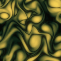
Before this paper a fluid solver had a speed limit: step too far and the simulation exploded, so the timestep was set by stability rather than by what anyone wanted to watch. Stam removed the limit by turning the question round. Instead of asking where a parcel of fluid goes, ask where the fluid now at this cell came from — trace the velocity backwards one whole timestep and read the field there, interpolating between the four cells the trace lands in. An average of four numbers is never larger than the largest of them, so that step cannot amplify anything, at any timestep at all; the dial here is a slider for exactly that reason, and it was measured to eight times its own ceiling without the field growing. What the method pays instead is blur. The same averaging that makes it stable smooths the flow a little every step, so a fluid left alone runs down, and this plate is stirred every second or so rather than pretending otherwise. Then the field is made incompressible, which is the other half: Helmholtz and Hodge say any vector field splits into a divergence-free part and a gradient, so subtracting the gradient of a pressure that solves one Poisson equation leaves precisely the part a fluid is allowed to have. Stam solved that equation with a Fourier transform on a wrapped domain; a lattice stepped one pass at a time has no transform to reach for, so this one relaxes it with twenty Jacobi sweeps a frame, warm-started from the last frame. The same equation, a slower solver, and the residual it leaves is printed in the console every time the plate gusts. What you see is the vorticity of the velocity field itself — bright where the flow curls, black where it is smooth — so the cores and the filaments strained off them are the fluid rather than a dye added to reveal it.

PROVENANCE

Origin

J. Stam, "Stable Fluids", Proceedings of the 26th Annual Conference on Computer Graphics and Interactive Techniques (SIGGRAPH 99), ACM Press, 1999, 121–128. Reprinted in Seminal Graphics Papers: Pushing the Boundaries, Volume 2, ACM, 2023, 779–786 (doi:10.1145/3596711.3596793)

Standing

Public domain — the Navier–Stokes equations are nineteenth century and the scheme is a published numerical method. Implemented here from the method as the paper sets it out, never from any fluid solver source

The projection, honestly

Stam projects in Fourier space on a periodic domain. A lattice advanced one shader pass at a time has no transform, so this plate solves the same Poisson equation by Jacobi relaxation instead, warm-started from the previous frame — and the residual is measured rather than assumed. At the published constants the divergence left in the field is 13 percent of its own vorticity in rms; the sweep count stops improving that at about fourteen, because Jacobi carries information one cell per sweep and what is left is long-wavelength. Measured across lattice sizes at a fixed twenty sweeps, the residual runs 2.2 percent at 96 cells and 8.4 percent at 256, so the lattice dial trades resolution against how incompressible the flow actually is. Both numbers are printed on every gust

The discrete decomposition

The divergence takes backward differences and the gradient forward ones. On a wrapped lattice those two are negative adjoints, so their composition is exactly the five-point Laplacian the sweeps invert and the split is orthogonal: the residual falls toward zero rather than toward a floor. Measured on a single field at 4,000 sweeps it reaches 0.07 percent of the divergence it was given, against 0.65 percent for central differences on both sides. At any sweep count this plate can afford the two are indistinguishable — the pairing is the right operator, not a visible improvement

Stability, measured

Advection alone, with no projection, was run 400 cycles from a field of peak speed 0.98: the peak falls to 0.18 at a timestep of 1 and to 0.007 at a timestep of 40, and never grows — which is the claim the paper makes, reproduced. The plate as a whole holds to a timestep of 16 at both ends of the viscosity slider and at every sweep count tried, on both the GPU and the JS path. The slider stops at 2.0, with margin

The forcing is ours

Stam wrote the equations; the eddies are a schedule added here so the plate has something to swirl, and they are a staging decision rather than published mathematics — the same admission ripple makes about its rain. Each eddy is a Gaussian patch of rotation, which has zero divergence analytically, so an impulse does not fight the projection that follows it

Constants

The timestep is a slider because the method does not need it to be small. Viscosity is the blend toward the neighbour average and mostly decides how long fine filaments survive against the blur the scheme itself adds. The sweep count is the quality of the projection and shows up in the number the gust prints rather than in the picture. The lattice is resolution here and not pattern scale — a fluid has a continuum limit, so the same flow appears finer rather than different, which is the opposite of what the Gray–Scott dial does

Source

doi:10.1145/311535.311548