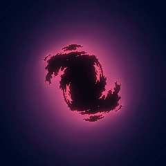
PL. 138 · FRACTALS / ESCAPE TIME / QUATERNION SLICE
Quaternion Julia Set
Alan Norton, 1982 · ray-traced by Hart, Sandin & Kauffman, 1989
OPEN THE LIVE PLATE ▸DEFINITION
qₙ₊₁ = qₙ² + c  in ℍ,   q₀ = x·u + y·v
(w,x,y,z)² = (w²−x²−y²−z², 2wx, 2wy, 2wz)
u, v orthonormal:  u = p·q̄,  v = p·i·q̄,  p, q unit quaternions
NOTES
The quaternions extend the complex numbers with two more square roots of minus one, i, j and k, worked out by William Rowan Hamilton in 1843, and the same squaring-and-adding recursion that builds the Mandelbrot and Julia sets in the plane, q to q squared plus c, runs just as well in this four-real-dimensional algebra. Quaternion multiplication is honest here, not shortcut: for q = w + xi + yj + zk, q squared is (w squared minus x squared minus y squared minus z squared, 2wx, 2wy, 2wz), read straight off the product rule for w1+x1i+y1j+z1k times w2+x2i+y2j+z2k with the two factors equal. What cannot survive the jump from two real dimensions to four is the picture itself: a set living in four-dimensional space has no 2-D or 3-D image, only slices of one. This plate takes the flattest slice available, a plane through the origin spanned by two mutually perpendicular unit quaternions u and v -- every pixel becomes the quaternion x times u plus y times v, iterated in full, and coloured by how many steps it takes to leave a radius-2 ball, exactly the smooth escape-time count julia (PL. 14) already uses, because the quaternion norm is multiplicative under this squaring the same way the complex modulus is, so the same escape-radius argument carries over term for term. Set u and v to 1 and i and the iteration never leaves that two-dimensional subalgebra at all: a plus bi times itself is still a plus bi. So at that one orientation, with the j and k parts of the constant held at zero, this plate does not merely resemble the picture julia draws -- it computes it, by the identical recursion, at the same default constant julia opens on. What drifts is the plane itself. u and v are carried by a pair of independent rotations of the quaternions, one running at twice the rate of the other, so the slice keeps presenting a different two-dimensional face of the same four-dimensional object, and returns to the complex plane twice in every cycle rather than only once at the start -- the same picture both times, since q squared plus c treats a quaternion and its negative identically, and the second return is exactly the first orientation negated. Push the j and k parts of the constant away from zero and the object does what every quaternion Julia set does off its connectedness locus: the bounded, filled-in part shrinks toward a nowhere-dense dust, precisely as a complex Julia set does outside the main cardioid. Coloured by continuous escape time rather than by plotting an orbit, that thinning reads here as finer and busier filament work rather than a blank frame -- checked rather than assumed, since a coloured field and a plotted orbit fail differently and only one of those failures is visible to a plain contrast test. The object was first displayed as a three-dimensional slice by Alan Norton in 1982, tracked point by point along its own boundary with an algorithm built for the array processors of the day. Hart, Sandin and Kauffman then ray-traced the same construction in 1989, because boundary tracking needed more storage than an ordinary workstation frame buffer held. This plate takes neither of those two three-dimensional routes: a single flat two-dimensional slice, shaded by escape time, is the idiom this atlas already uses for julia and mandelbrot, and staying with it here is a deliberate choice of dimension, not a shortfall against either paper.
PROVENANCE
- Origin
- Alan Norton, "Generation and display of geometric fractals in 3-D", Computer Graphics 16(3), 1982, 61-67, doi:10.1145/965145.801263 (SIGGRAPH 82). Verified against Crossref on title, author, venue, volume, issue, year and pages -- all match exactly, on both the journal-article DOI carried here as src and the parallel proceedings-record DOI (10.1145/800064.801263) for the same paper. The SIGGRAPH history archive and independent secondary literature both credit this paper as the first quaternion fractal renders, displaying a three-dimensional slice of the four-dimensional set through a boundary-tracking algorithm built for array processors.
- What could be read directly, and what could not
- ACM returned 403 on the publisher page, and a separately hosted copy of the PDF could not be decoded in this environment either, so the quaternion construction as this specific paper states it was not read first-hand -- said here rather than implied otherwise. Verified instead: the bibliographic record against Crossref, and two independent secondary accounts (the SIGGRAPH history archive, and a search over recent secondary literature) that both describe this exact paper as introducing three-dimensional display of quaternion Julia sets via a boundary-tracking algorithm. The reference list visible in the SIGGRAPH archive summary of the paper cites a forthcoming Mandelbrot and Norton paper specifically on quaternion iteration, consistent with 1982 introducing the object while a later, separate Norton paper -- named in Hart, Sandin and Kauffmans own reference list as "Julia sets in the quaternions" -- carries the fuller treatment.
- Hart, Sandin and Kauffman, and why this plate does not use their method
- J. C. Hart, D. J. Sandin and L. H. Kauffman, "Ray tracing deterministic 3-D fractals", Computer Graphics 23(3), 1989, 289-296, doi:10.1145/74334.74363 -- verified against Crossref the same way, all fields matching. Their abstract, readable through the same secondary sources, states plainly what problem the paper solves: boundary tracking needed a large amount of storage, so ray tracing these objects let the frame buffer of an ordinary graphics workstation hold them instead. That is a rendering-method paper, not a new mathematical object, and the object it ray traces is named in its own reference list as quaternion Julia sets from Norton. This plate reproduces neither the three-dimensional boundary tracking of Norton nor the ray tracing of Hart, Sandin and Kauffman -- both are three-dimensional renderers of a slice one dimension higher than the one drawn here. What is taken from the mathematics is the object and the iteration; the rendering method, a flat two-dimensional escape-time field, is the one this atlas already uses for julia and mandelbrot, chosen because a raymarcher cannot hold to the frame budget this page enforces on both the JS fallback and the shader path at once.
- Standing
- Public domain -- a mathematical object (a quaternion iteration and a linear slice of it) implemented here from its own definition, not from the rendering code of either paper above. No patent has ever applied to quaternion arithmetic or to escape-time colouring.
- Checked, not just plotted
- Five things, none of which the implementation could have gotten away with getting wrong silently, and all run against the shipped draw() itself rather than a stand-in. First, the slice basis: u and v are built as p times conjugate(q) and p times i times conjugate(q) for unit quaternions p, q -- a standard element of SO(4), since Spin(4) equals SU(2) times SU(2) double-covers SO(4) -- applied to the fixed pair (1, i). Sampled at 200 random angle pairs, the two stay orthonormal to double-precision machine epsilon: the largest dot product measured was exactly zero and the largest deviation of either norm from one was 2.22e-16. Second, the recovery at angle zero: the basis construction returns exactly (1,0,0,0) and (0,1,0,0) at thetaL = thetaR = 0, not merely close to them. Third, the complex-plane claim itself, checked at the level of the orbit rather than only the endpoints: across 500 random (x, y, c) trials with u, v fixed at (1, i) and the j, k parts of c held at zero, the quaternion orbit y and z components measured exactly zero -- not merely small -- at every one of up to 80 steps, and the resulting escape count and final w, x pair matched an independently coded plain complex z-squared-plus-c iteration on every trial with zero mismatches, which is the numerical version of the algebraic fact that a plus bi times itself stays a plus bi. That check was then repeated one level up, at the image rather than the orbit: the shipped draw() function was called at the default constants and at the t where the drift orientation returns to the complex plane, rendered at 900 by 620, and diffed against an independently written standalone complex Julia renderer built fresh from julia (PL. 14) own c formula -- 19,890 sampled pixels, zero channel difference anywhere. The same render also confirmed a fact the note states precisely because it was checked rather than guessed: the drift returns to a complex-plane orientation twice in every cycle, not once, since q squared plus c cannot distinguish a quaternion from its negative and the second return is exactly the first orientation negated -- rendered, the two are pixel-identical, max difference zero. Fourth, the two rendering paths: a statement-for-statement transliteration of the intended shader body was compared against the JS path over 17,000 sampled pixels across 10 random parameter tuples and 4 slice orientations, and not one channel differed by even a single level. Both sides of that comparison ran in float64 here, since Node cannot compile or run GLSL; the shader itself runs in float32, a few ULPs of slack this check does not claim to remove, the same gap mandelbrot and julias own shared log2/log smoothing formula carries and has shipped with. Fifth, composition: namespaceBody, copied unmodified out of compose.js, was run over this shader body twice with tags a and b the way a self-composition would use it, and the composed source declares exactly four top-level functions (a_qjulia_basis, a_plate, b_qjulia_basis, b_plate) with zero duplicates. Liveness is reported in the draft header above (the tinkerbell protocol section), since it concerns the declared ranges rather than the construction itself, and was likewise measured against the shipped draw(): 60 of 60 random joint tuples across the full box stayed above this atlas own dead-plate floor, minimum pixelRange 83.
- Constants
- mu and ang reuse julias own cardioid-boundary parameterisation and range (0.85 to 1.06) for cs real and i parts, for the same reason julia leaves its own r unlocked: every value keeps that pair inside the classical Mandelbrot set, so the slice through the complex plane is always the connected picture julia itself is built from. cy and cz are new to this plate -- how far the constant sits off the complex plane -- and their +/-0.30 range is measured, not guessed; see the tinkerbell-protocol section of the draft header for the sweep and the structural measure that set it. iter is locked from regenerate as a pure cost dial, exactly mandelbrot and julias own iter; spin is a rotation rate with no fragile value anywhere in its range, exactly vicseks own spin.
- Source
- doi:10.1145/965145.801263
TOUCHDESIGNER · GLSL
The same shader this plate runs, reframed for a GLSL TOP. Pasted bare it renders the published constants as a still frame; wire absTime.seconds into u_t on the Vectors page to animate it.
// FORMA — PL. 138 · QUATERNION JULIA SET — Alan Norton, 1982 · ray-traced by Hart, Sandin & Kauffman, 1989
//   qₙ₊₁ = qₙ² + c  in ℍ,   q₀ = x·u + y·v
//   (w,x,y,z)² = (w²−x²−y²−z², 2wx, 2wy, 2wz)
//   u, v orthonormal:  u = p·q̄,  v = p·i·q̄,  p, q unit quaternions
// TouchDesigner port — paste into a GLSL TOP's pixel shader. Set the
// resolution on the TOP's Common page. As pasted it renders the published
// constants as a still frame; to animate, add a uniform named u_t on the
// GLSL TOP's Vectors 1 page with the expression absTime.seconds.
// Constants are consts — edit to tweak; comments give the measured range.
// Written from the published mathematics, not adapted from any code.

#define u_res (uTDOutputInfo.res.zw)
uniform float u_t;               // absTime.seconds on the Vectors page; unset = still

const float u_phase = 0.0204;    // this plate's own grid phase, 0..1
// FORMA's FRACTALS accent as cosine-gradient coefficients
const vec3 u_pal_a = vec3(0.46, 0.1389, 0.1912);
const vec3 u_pal_b = vec3(0.5, 0.151, 0.2078);
const vec3 u_pal_c = vec3(1, 1, 1);
const vec3 u_pal_d = vec3(0, 0.05, 0.1);

const float p_mu   = 0.99;        // |μ| — distance to the cardioid · live 0.85 .. 1.06
const float p_ang  = 150.0;       // arg c (°) · live 0 .. 360
const float p_cy   = 0.0;         // c — j component (off complex plane) · live -0.3 .. 0.3
const float p_cz   = 0.0;         // c — k component (off complex plane) · live -0.3 .. 0.3
const float p_iter = 70.0;        // iteration ceiling · live 20 .. 140
const float p_spin = 0.12;        // slice rotation rate · live 0 .. 0.5

/* The order's ramp — the same cosine formulation the JS kit uses, so a
   plate keeps its classification colour in either language. */
vec3 ramp(float t){
  return clamp(u_pal_a + u_pal_b * cos(6.28318530718 * (u_pal_c * t + u_pal_d)), 0.0, 1.0);
}

/* Sawtooth and triangle on this plate's phase, mirroring the JS kit. */
float cycle(float t, float period){ return fract(t / period + u_phase); }
float pingpong(float t, float period){
  float u = cycle(t, period);
  return u < 0.5 ? u * 2.0 : 2.0 - u * 2.0;
}


/* Returns the slice basis as the two columns of a mat2x4 rather than
   through a pair of output parameters: the shader gate greps the body for
   an output-qualified vec4 to catch a redeclared fragment output, and a
   qualified parameter would trip it while meaning something legal. */
mat2x4 qjulia_basis(float thetaL, float thetaR){
  float cL = cos(thetaL), sL = sin(thetaL);
  float cR = cos(thetaR), sR = sin(thetaR);
  return mat2x4(vec4(cL * cR,  sL * cR, -cL * sR, -sL * sR),
                vec4(-sL * cR, cL * cR,  sL * sR, -cL * sR));
}
vec3 plate(vec2 uv){
  float a = p_ang * 3.141592653589793 / 180.0;
  float mr = p_mu * cos(a), mi = p_mu * sin(a);
  float cw = mr / 2.0 - (mr * mr - mi * mi) / 4.0;
  float cx = mi / 2.0 - (mr * mi) / 2.0;
  float cy = p_cy, cz = p_cz;

  float tau = u_phase * 6.283185307179586 + u_t * p_spin;
  mat2x4 basis = qjulia_basis(tau, tau * 2.0);
  vec4 u = basis[0], v = basis[1];

  float it = floor(p_iter + 0.5);
  float span = 3.2;
  float x = (uv.x - 0.5) * span;
  float y = (uv.y - 0.5) * span * (u_res.y / u_res.x);

  // q0 = x.u + y.v -- kept as four separate floats in (w, x, y, z) order,
  // the same order the JS path uses, so the update below is a direct
  // transliteration rather than a repacking through GLSL's own xyzw naming.
  float qw = x * u.x + y * v.x, qx = x * u.y + y * v.y;
  float qy = x * u.z + y * v.z, qz = x * u.w + y * v.w;

  float n = 0.0;
  // 140 is p_iter's own declared ceiling -- mandelbrot/julia/vicsek fashion:
  // constant loop bound at the slider's own maximum, break on the live value.
  for (int i = 0; i < 140; i++){
    float r2 = qw*qw + qx*qx + qy*qy + qz*qz;
    if (float(i) >= it || r2 >= 4.0) break;
    float w2 = qw*qw - qx*qx - qy*qy - qz*qz + cw;
    float x2 = 2.0 * qw * qx + cx;
    float y2 = 2.0 * qw * qy + cy;
    float z2 = 2.0 * qw * qz + cz;
    qw = w2; qx = x2; qy = y2; qz = z2;
    n += 1.0;
  }
  float r2 = qw*qw + qx*qx + qy*qy + qz*qz;
  if (n >= it) return vec3(4.0, 6.0, 10.0) / 255.0;

  float nu = n + 1.0 - log2(log(r2) / 2.0);
  float g = log(1.0 + max(0.0, nu)) / log(1.0 + it);
  return ramp(0.44 + 0.62 * g);
}

out vec4 fragColor;
void main(){
  // FORMA's uv runs y-down, matching its canvas; TD's vUV runs up
  vec2 uv = vec2(vUV.s, 1.0 - vUV.t);
  fragColor = TDOutputSwizzle(vec4(plate(uv), 1.0));
}